THE FIVE DEVELOPMENT AXES

Body, feeling, attention, language and sensory blindness

Version 11 — Fully illustrated with 110+ charts

Parenting crisis, AI transition, industrial decline and talent outflow

Each chart described and supported

Jacobus van Merksteijn — September 2026

Reading guide v11

This is the tenth full version of an integrated analysis of four loss episodes simultaneously affecting the Netherlands: parenting crisis, AI labor-market transition, industrial decline and talent outflow. In v11 all available charts from earlier sessions have been included, each with description, methodology and source citation.

New in v11 compared with v10:

• Complete chart set from all research batches (110+ charts)

• Each chart provided with description + methodology + source

• Charts thematically organized by analytical lens

• New scenario names (Short-circuit, Shock approach, Media brake, Nature boarding schools, Integrated parenting chain, Future-oriented parenting chain, Dutch Renaissance) in the text; old scenario charts still show the letter (equivalence indicated)

Scenario translation table:

Old letter (in chart)	New name (in text)
K base	Short-circuit
K + re-entry	Short-circuit plus
H shock	Shock approach
I media levy	Media brake
Boarding schools only	Nature boarding schools
M integrated	Integrated parenting chain
N (M+AI)	Future-oriented parenting chain
O change of course	Dutch Renaissance

Chart convention in v10 charts (Parts B through F):

• Measured data — Dark color + solid line + filled circles

• Forecast — Light color + dotted line + open circles

• Separation — Gray vertical dotted line

Part A — The five development axes

A.1 Five axes summarized

Axis	Core	Formation window	Strongest causes of failure
1. Body	motor skills, strength, endurance	0–7 years (first solidification phase)	No outdoor play
2. Feeling	attachment, empathy, self-regulation	0–7 years	Childcare + mother works
3. Attention	focus, concentration	0–7 years (first solidification phase)	Screen time
4. Language	verbal expression, reading, analysis	7–14 years	Screen time + education
5. Sensory blindness	3D capacity: depth perception + depth motor skills + stereometric cortex + stereometric thinking + danger-and-boundary awareness	0–7 years foundation, reinforcement 7–14 years through play and experience	Screen time + no outdoor play + no 3D construction

A.2 Five development axes by birth cohort

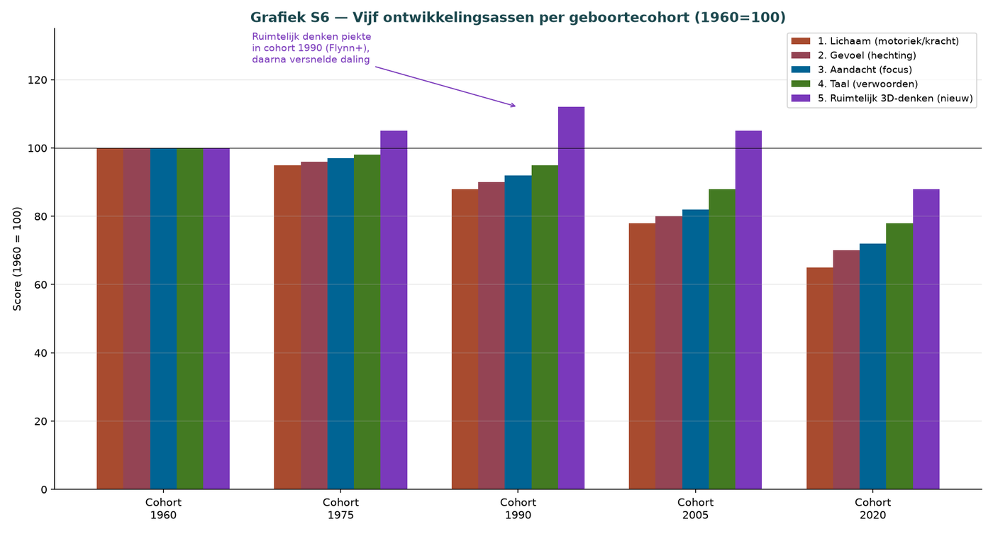
Description: All five axes decline from cohort 1975 onward, with the exception of spatial 3D thinking, which peaks in cohort 1990 (Flynn peak). From cohort 2005 onward, the decline accelerates on all axes. Cohort 2020 is at 65 to 88% of the 1960 level.

Method: Each axis normalized to 100 for birth cohort 1960. Values for 1975/1990/2005/2020 per axis derived from measurement sources: KOMBO motor skills (axis 1), family stability index (axis 2), NEA focus (axis 3), PIRLS/PISA (axis 4), 3D cubes + PISA spatial-form (axis 5).

Source: Compilation of CBS, OECD PISA, Pietschnig 2015 (Flynn 3D cubes), Erasmus MC.

Overview chart of all five development axes by birth cohort, with 1960 as the reference point (=100). Cohorts 1960/1975/1990/2005/2020 on five axes. Spatial 3D thinking peaked in cohort 1990 (Flynn peak), after which decline accelerated on all axes. Cohort 2020 is at 65 to 88% of the 1960 level. Cohort 2020 is now entering VMBO/HAVO/VWO (solidification phase S3, 14–21 years) and will later enter HBO/WO (S4, 21–35 years). All five axes simultaneously below the 1960 level means that every further education program must work with fewer basic skills. [Source: Position Paper to the Tweede Kamer on PISA reading literacy (2024, 2024D10790), Pietschnig & Voracek, meta-analysis of the Flynn effect (2015)]

A.3 Five components of sensory blindness

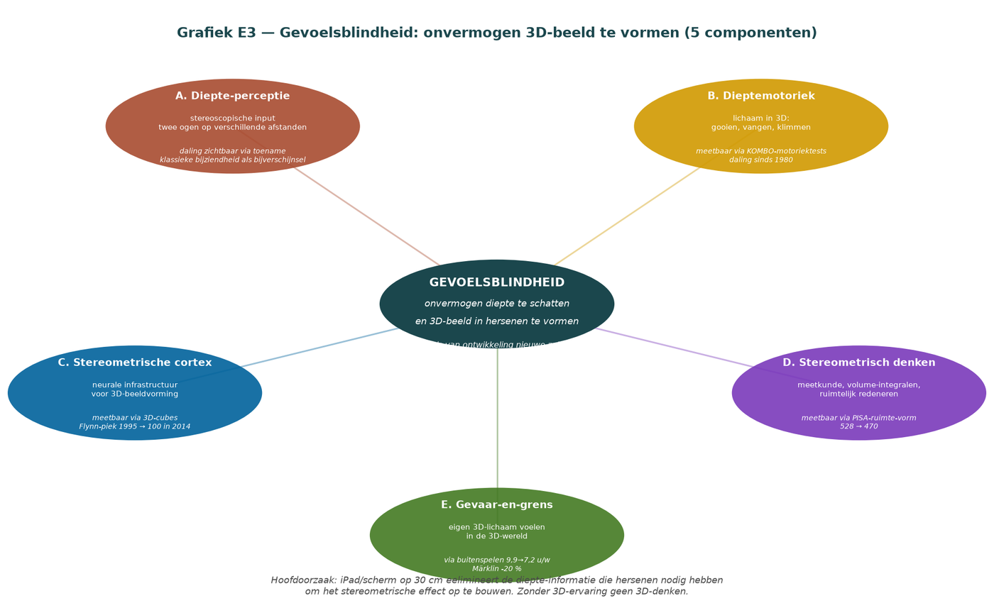
Description: Sensory blindness is the interconnected function-axis from depth perception to depth thinking to risk assessment. Loss of depth perception is a SYMPTOM of the same mechanism, not the problem itself.

Method: Five components (each weighted 20% in composite score): A depth perception (stereoscopic input), B depth motor skills (KOMBO), C stereometric cortex (Flynn 3D cubes), D stereometric thinking (PISA spatial form), E danger-and-boundary awareness (outdoor play, construction toys).

Source: Synthesis of this report.

Definition diagram of sensory blindness as the fifth axis with five components (A through E). Sensory blindness = inability to estimate depth and form a 3D image in the brain. Main cause: iPad at 30 cm eliminates depth input during solidification phase S1 (0–7 years) and S2 (7–14 years). Classic myopia = symptom, not the problem. Component D (Stereometric thinking) manifests in solidification phase S3 (14–21 years) as mathematics education; at university (S4, 21–35 years) as beta-technical education. Without an S1+S2 foundation, S3 and S4 cannot be filled. [Source: TU Delft, ‘Solving the shortage of engineers requires a talent strategy’ (2026)]

The five components:

• A. Depth perception — stereoscopic input from two eyes at different distances — the physical input from which the brain constructs 3D

• B. Depth motor skills — moving the body in 3D: throwing, catching, jumping, climbing

• C. Stereometric cortex — neural infrastructure for 3D imaging: visual cortex, parietal cortex, 3D navigation hippocampus, systems thinking in the prefrontal cortex

• D. Stereometric thinking — cognitive application of 3D capacity: geometry, stereometry, volume integrals, tensors, spatial reasoning

• E. Danger-and-boundary awareness — feeling one's own 3D body in the 3D world: physical risk assessment, understanding of materials, sense of consequences

Part B — Four classic parenting causes

B.1 Childcare — main chart v10

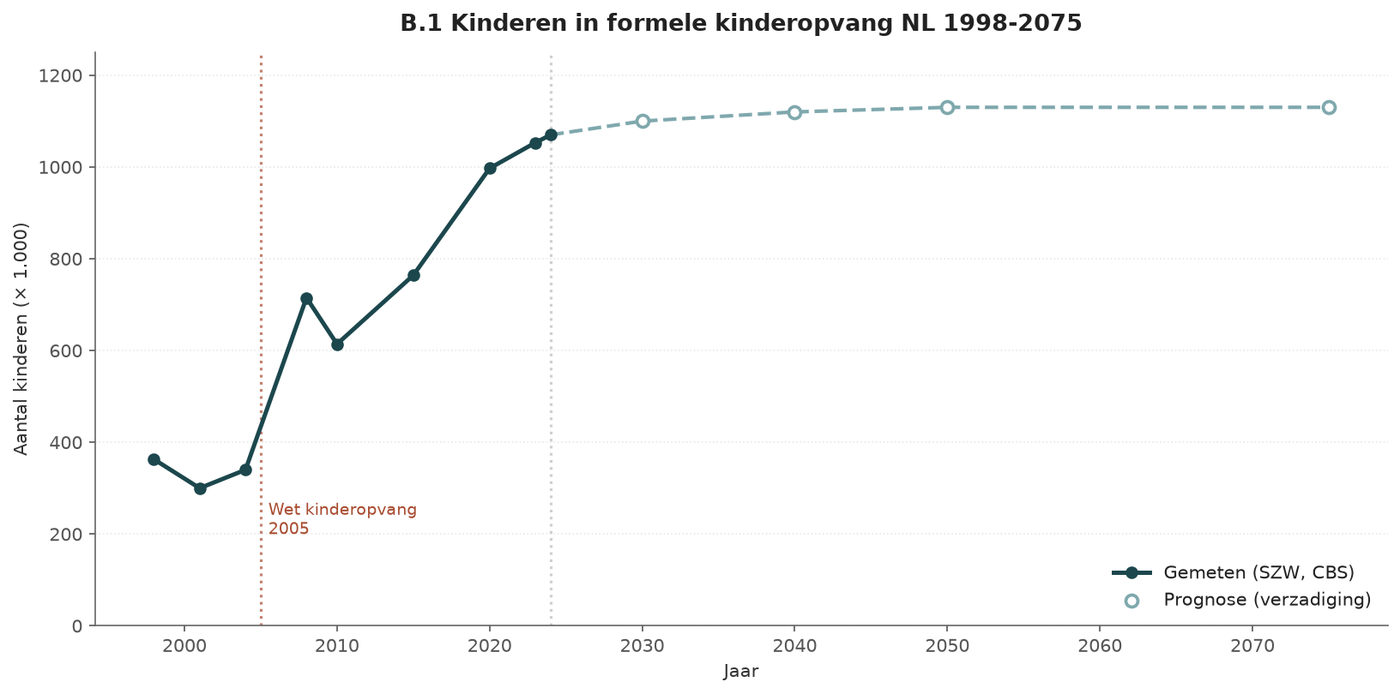
Description: From 300 thousand (2001) to 1.07 million children (2024). Childcare Act 2005 as a turning point. Forecast levels off at around 1.13 million under unchanged policy.

Method: Measured data from SZW quarterly reports 1998–2024. S-curve forecast with saturation based on the demographic peak of the Netherlands.

Source: SZW Quarterly Childcare Reports, CBS.

Basic childcare series: fundamental demographic shift affecting solidification phase S1 (0–7 years). From 300 thousand (2001) to 1.07 million children in formal childcare (2024). Childcare Act 2005 as a turning point. Manifestation in S1: children spend the most important solidification phase in a standardized 2D environment. The Education Council recommends early childhood education for at-risk children aged 0–7, but at the same time signals attachment risk among non-risk groups. [Source: Onderwijsraad, ‘Advisory letter on provisions for young children’ (2023)]

B.4 Maternal employment

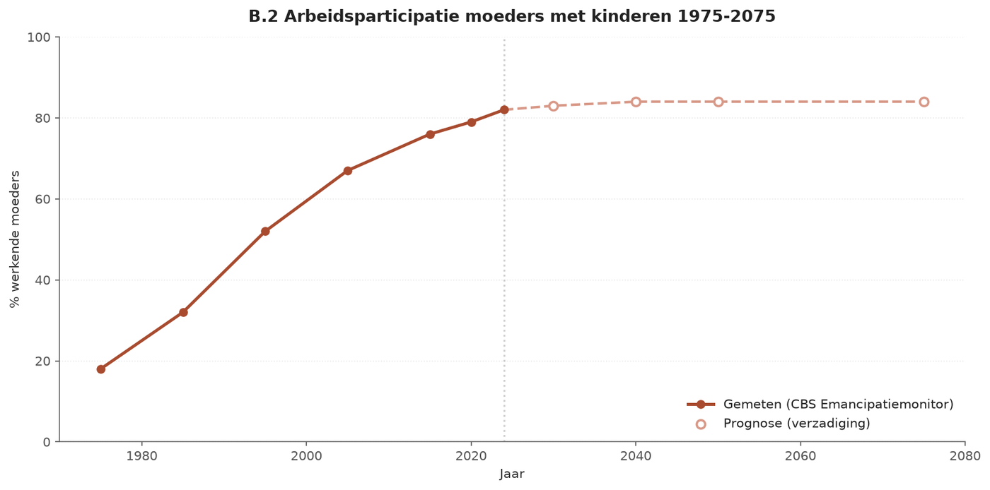
Description: From 18% (1975) to 82% (2024) — the fundamental demographic change. Forecast levels off at around 84%.

Method: CBS figures for mothers aged 21–35 (S4) to 35–77 (S5) years with at least one minor child.

Source: CBS Emancipation Monitor.

Fundamental shift in maternal employment 1975–2075. From 18% (1975) to 82% (2024). Doubling between 1975 and 1995, leveling off at around 84%. A working mother means that S1 (0–7) largely takes place in childcare. Direct connection to educational performance is not explicit in OCW reports; model-based through axis 2 (Feeling), carrying through to S4 (working life). [Model-based transmission via Appendix 1]

B.6 Screen time

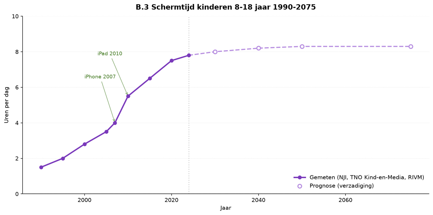
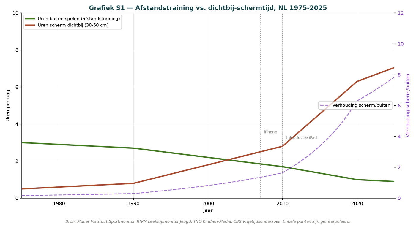
Description: From 1.5 hours/day (1990) to 7.8 hours/day (2024). iPhone 2007 and iPad 2010 as turning points. Forecast levels off at around 8.3 hours/day.

Method: Aggregation of NJI media research, TNO Children and Media five-year surveys, RIVM Youth Monitor.

Source: NJI, TNO Children and Media, RIVM.

Screen time as a central cause in the influence model: affects S1 (0–7) and S2 (7–14). From 1.5 hours/day (1990) to 7.8 hours/day (2024, cohort aged 7–21). iPhone 2007 and iPad 2010 as turning points. Forecast levels off at around 8.3 hours/day. An iPad at 30 cm during S1 blocks depth-perception training (component A of sensory blindness). AJN youth physicians explicitly warn about myopia and concentration problems. In S2 (7–14), screen time displaces play and experiences through which 3D capacity would be strengthened. [Source: AJN Youth Physicians, ‘Fact sheet: screen use at close range’ (2019), TNO, Pluymen et al., ‘Screen use’ (2024)]

B.8 Digital media use by young children aged 0–7

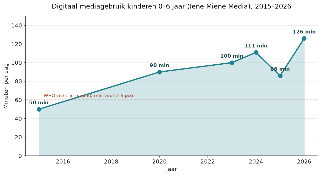
Description: From 50 min/day (2015) to 126 min/day (2026). The WHO guideline of a maximum of 60 minutes for ages 0–7 is exceeded from 2018 onward and continues to rise.

Method: Sample of parents of children aged 0–7, current measurement of the previous day.

Source: Iene Miene Media research, Netwerk Mediawijsheid NL, every 2–3 years.

Measurement of the youngest age group, 0–7 years — crucial for sensory blindness component A and attention in S1. From 50 min/day (2015) to 126 min/day (2026). The WHO guideline of a maximum of 60 minutes for ages 2–5 is exceeded from 2018 onward and continues to rise. AJN youth physicians: ‘For children up to age 2, screen use should be limited as much as possible; up to age 5, maximum 1 hour per day.’ The actual 126 minutes is far above this. These cohorts will soon enter S2 with a disrupted S1 foundation. [Source: AJN Youth Physicians, ‘Fact sheet: screen use at close range’ (2019)]

B.9 Teacher shortage

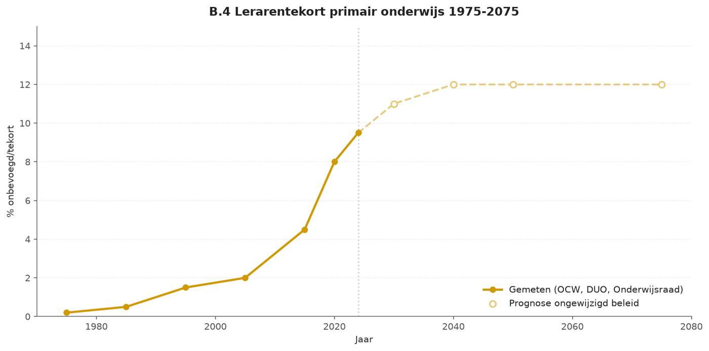
Description: From 0.2% (1975) to 9.5% (2024) unqualified or vacant. Forecast stabilizes at around 12% under unchanged policy.

Method: OCW qualification registration + DUO vacancy monitor + Onderwijsraad estimate.

Source: OCW, DUO, Onderwijsraad.

Teacher shortage in primary education 1975–2075: primarily affects solidification phase S2 (7–14 years), in which language and play would be reinforced. From 0.2% unqualified/shortage (1975) to 9.5% (2024). Forecast stabilizes at around 12%. Onderwijsraad (‘Scarcity hurts’ 2023): ‘At schools with a shortage above 10%, the percentage insufficient is highest.’ Direct connection between shortage and learning outcomes in the S2 phase. [Source: Onderwijsraad, ‘Scarcity hurts’ (2023), Inspectorate of Education, Technical report on teacher shortage (2024)]

B.11 Overview of four causes together (v10)

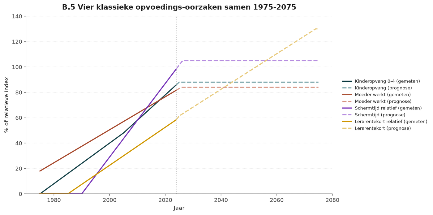
Description: Four causes on one axis with measured data (solid line) and forecast (dotted line). All four rise: childcare, maternal employment, screen time and teacher shortage.

Source: Combination of the sources above.

Overview chart: four classic causes on one axis show the simultaneity of changes affecting S1 and S2. Four causes 1975–2075. Measurement through 2024, forecast thereafter. All four causes act together on solidification phases S1 (0–7) and S2 (7–14), resulting in a cumulative effect on cohorts now in S3–S5. [Model-based transmission via Appendix 1]

B.13 Integrated parenting causes (extended)

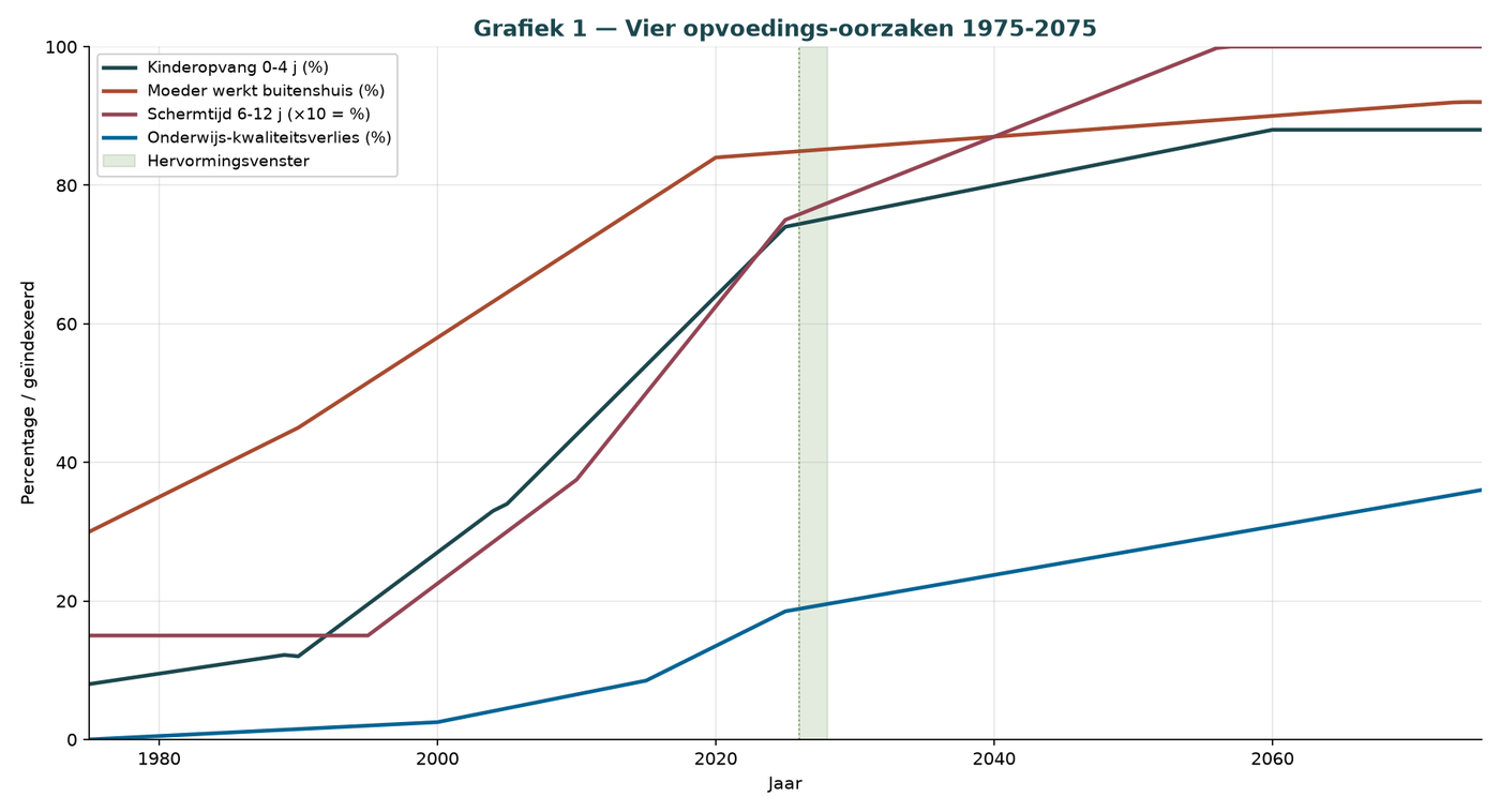
Description: Same four causes, but with scenario lines for Integrated parenting chain and Dutch Renaissance included as counter-scenarios.

Method: Scenario modeling: reduction of childcare participation to 15% and screen time to 3 hours/day as a target for the Integrated parenting chain.

Source: Modeling by CBS/OCW/NJI with scenario overlay.

Four parenting causes with scenario lines (Integrated parenting chain, Dutch Renaissance) as counter-scenarios. Adaptability through policy intervention: childcare to 15% (protects S1), screen time to 3 hours/day (protects S1+S2). Interventions aimed at S1 and S2 have an effect in S3–S5 with a delay of 14–35 years. [Model-based transmission via Appendix 1]

Part C — Measured outcomes

C.1 PISA reading proficiency — main chart v10

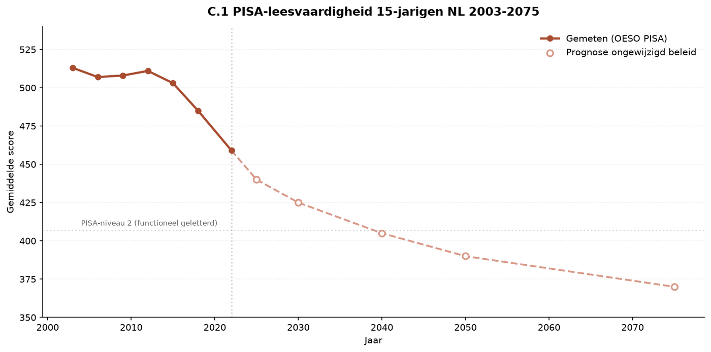
Description: From 513 (2003) to 459 (2022) — a decline of 54 points in 19 years. One of the strongest declines worldwide. Forecast falls below PISA level 2 around 2040.

Method: PISA assessment cycles: 2003, 2006, 2009, 2012, 2015, 2018, 2022. Forecast based on linear extrapolation with saturation at 370 around 2075.

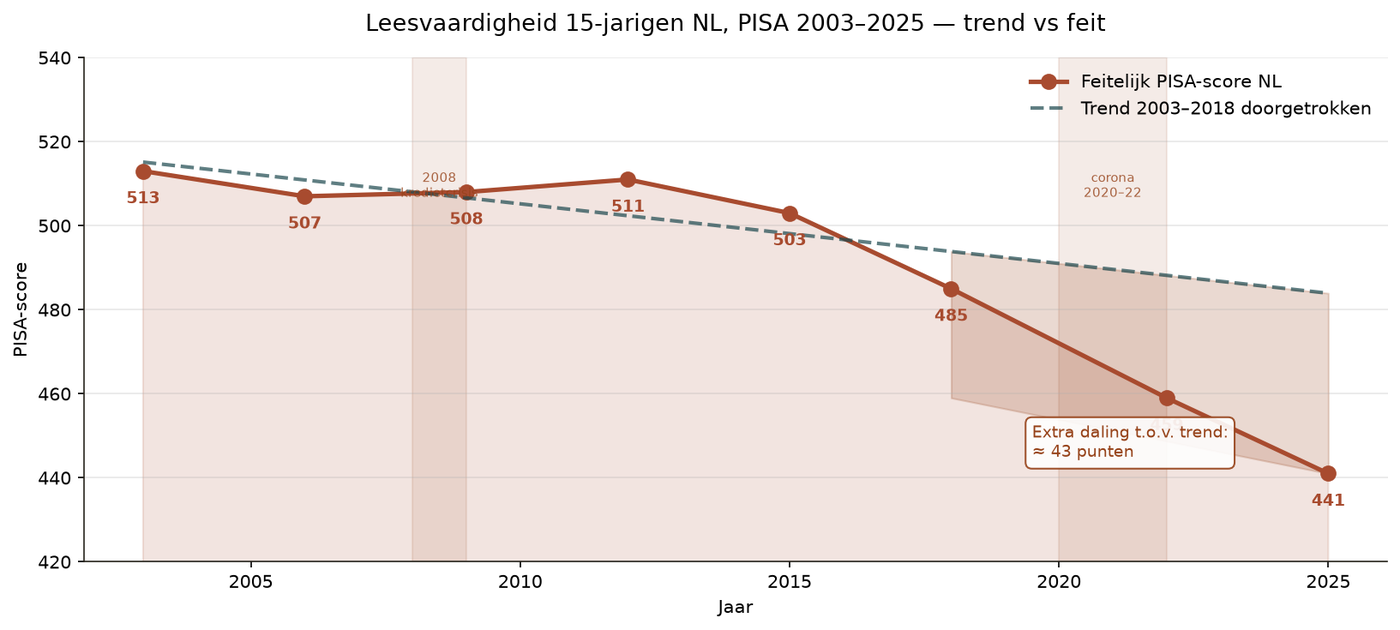
Source: OECD PISA. The PISA 2025 cycle has not yet been published (expected December 2026).

Central PISA chart: reading proficiency of 14-year-olds in the Netherlands. Measures outcome of solidification phase S2 (7-14). From 513 (2003) to 459 (2022), a decline of 54 points in 19 years. Forecast falls below PISA level 2 (functionally literate) around 2040. Position Paper of the Tweede Kamer (2024) calls the decline ‘exceptionally rapid’. PISA 2025 (July 2026) shows a further decline. These cohorts move on to S3 (14-21, secondary-school final examination) and S4 (21-35, higher education). Direct outcome: higher first-year HBO/WO dropout due to insufficient language proficiency. [Source: Position Paper of the Tweede Kamer on PISA reading proficiency (2024, 2024D10790), Expert Network for STEM Education, ‘Results PISA 2025’ (July 2026)]

C.2 PISA reading trend (long)

Description: NL decline compared with the OECD average and Finland. Finland is also declining but less sharply.

Method: Comparison of PISA scores over the same assessment cycles.

Source: OECD PISA.

International comparison of PISA reading: NL is declining faster than Finland and the OECD average. NL fell from above the OECD average to below average between 2015 and 2022. OECD PISA 2022 Country Note NL: ‘Average performance was lower in 2022 than in any previous assessment.’ [Source: OECD, PISA 2022 Country Note Netherlands]

C.4 PISA mathematics

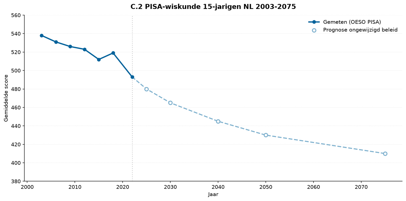
Description: From 538 (2003) to 493 (2022). Crucial for STEM education and industrial alignment.

Source: OECD PISA.

PISA mathematics among 14-year-olds in NL: crucial for STEM education. From 538 (2003) to 493 (2022), a decline of 45 points. TU Delft (2026): ‘The number of Dutch students choosing a technical degree is falling again.’ Mathematics proficiency from S2/S3 determines STEM intake in S4. [Source: TU Delft, ‘Addressing the shortage of engineers requires a talent strategy’ (2026)]

C.5 PISA space and shape

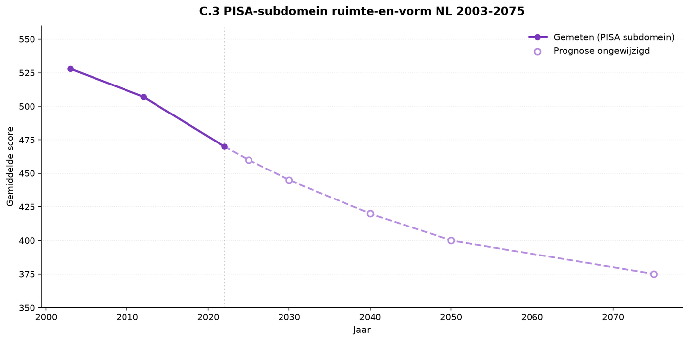
Description: From 528 (2003) to 470 (2022) — a 58-point decline. Strongest indicator for the cognitive component of sensory blindness (component D).

Method: PISA reports subdomain scores per assessment cycle.

Source: OECD PISA subdomain scores.

PISA space-and-shape subdomain: strongest direct indicator of the sensory blindness component D (stereometric thinking) in solidification phases S2/S3. From 528 (2003) to 470 (2022), a decline of 58 points — sharper than overall mathematics. This decline affects S4 (21-35) STEM programs that require stereometric reasoning: civil engineering, mechanical engineering, architecture, physics. [Source: OECD PISA subdomain scores]

C.6 PISA space-shape (stereo version)

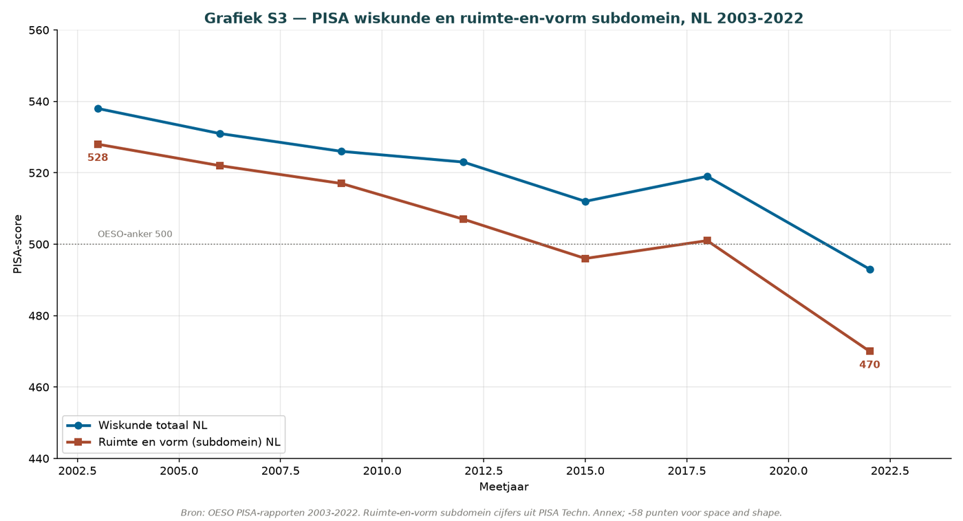
Description: Alternative visualization with comparison of OECD countries.

Source: OECD PISA subdomains.

Alternative visualization of PISA space-shape with OECD comparison. NL compared with OECD countries on the subdomain. Same educational implications as C.5. [Source: OECD PISA]

C.7 PISA scores across domains

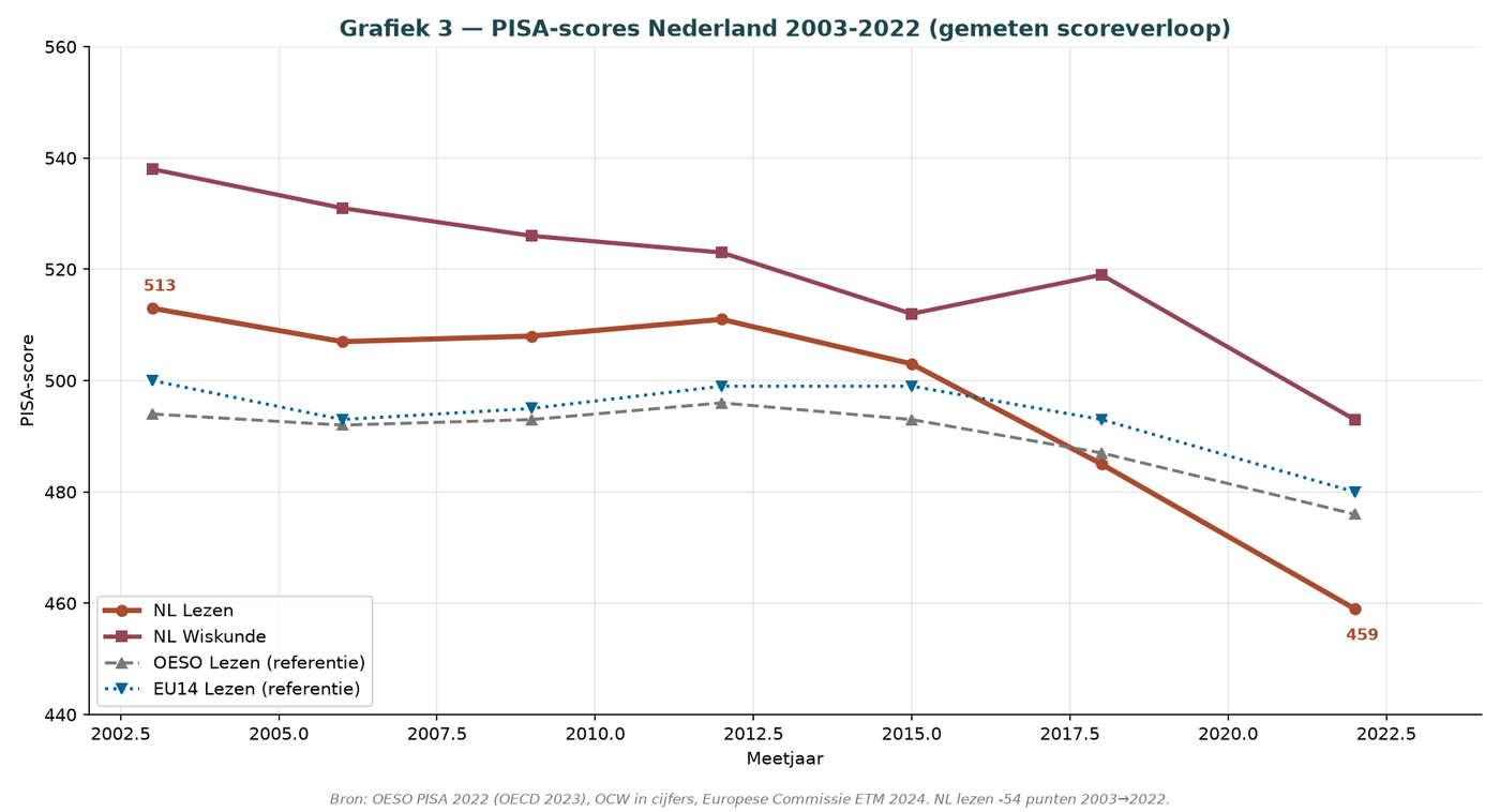
Description: All three domains on one axis: all three decline sharply after 2015. Science declines least.

Source: OECD PISA.

Multi-domain PISA view: reading, mathematics, and science together. All three decline sharply after 2015. Science declines least. Cumulative effect on all subsequent programs. [Source: Position Paper of the Tweede Kamer on PISA reading proficiency (2024, 2024D10790)]

C.8 PISA below level 2

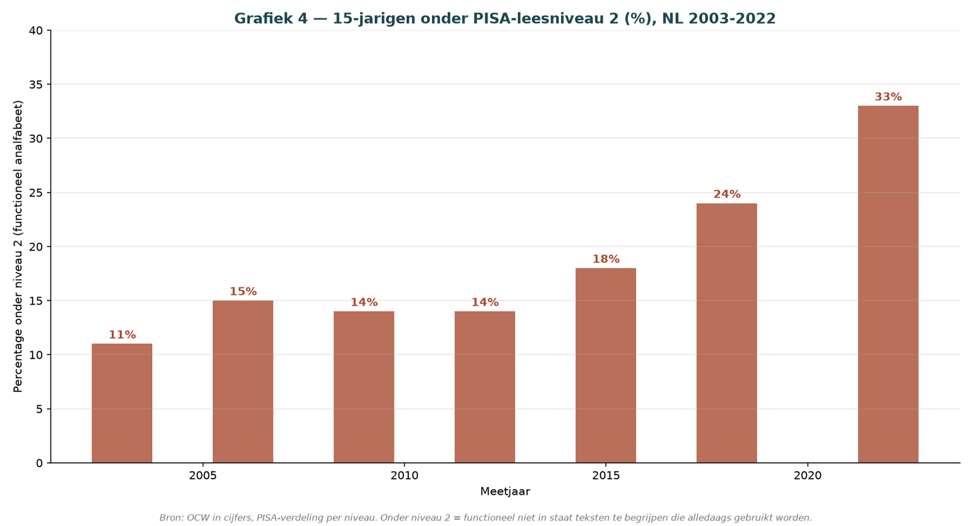
Description: Crucial: the proportion of functionally illiterate 14-year-olds grew from 12% (2003) to 33% (2022). One in three students cannot use text functionally.

Method: PISA level 2 is the OECD threshold for functional literacy.

Source: OCW in figures, OECD PISA.

Percentage of functionally illiterate 14-year-olds: most direct indicator of societal risk. From 12% (2003) to 33% (2022). One in three 14-year-olds cannot use text functionally. These students leave VMBO and HAVO as functionally low-literate; MBOs report needing more intake tests in reading. Direct effect on S3 and S4. [Source: Position Paper of the Tweede Kamer on PISA reading proficiency (2024, 2024D10790)]

C.9 PIRLS 7-14 cohort — v10 main chart

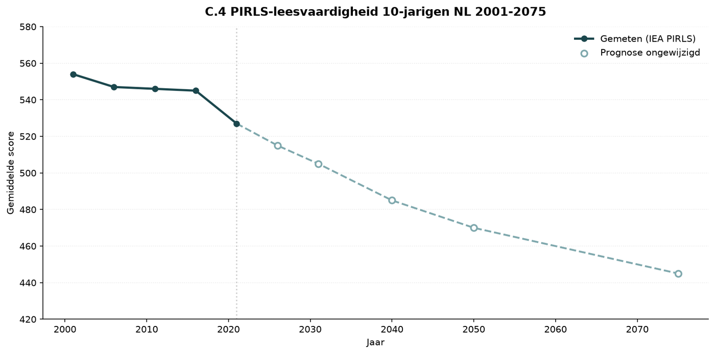
Description: From 554 (2001) to 527 (2021). PIRLS tests the 7-14 cohort, thus showing the cohort that was ~2011 in primary school.

Source: IEA PIRLS 2001, 2006, 2011, 2016, 2021.

PIRLS 7-14 cohort NL: earlier signal than PISA. Shows that the reading decline already emerges in solidification phase S2 (7-14). From 554 (2001) to 527 (2021). The PIRLS 7-14 decline predicts the PISA-14 decline 4-7 years later. Primary education (S2) must restore reading proficiency before secondary-school intake stabilizes. [Source: IEA PIRLS, Onderwijsraad, ‘Scarcity bites’ (2023)]

C.10 PIRLS long version

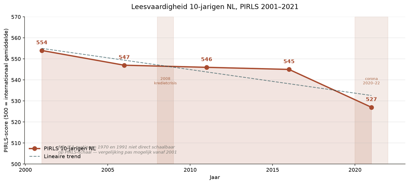
Description: NL fell from the top 3 (2001) to rank 25 (2021) in the international ranking.

Source: IEA PIRLS.

International PIRLS reading ranking: NL fell from the top 3 (2001) to rank 25 (2021). Loss of position internationally. Same as C.9. [Source: IEA PIRLS]

C.12 Burnout — v10 main chart

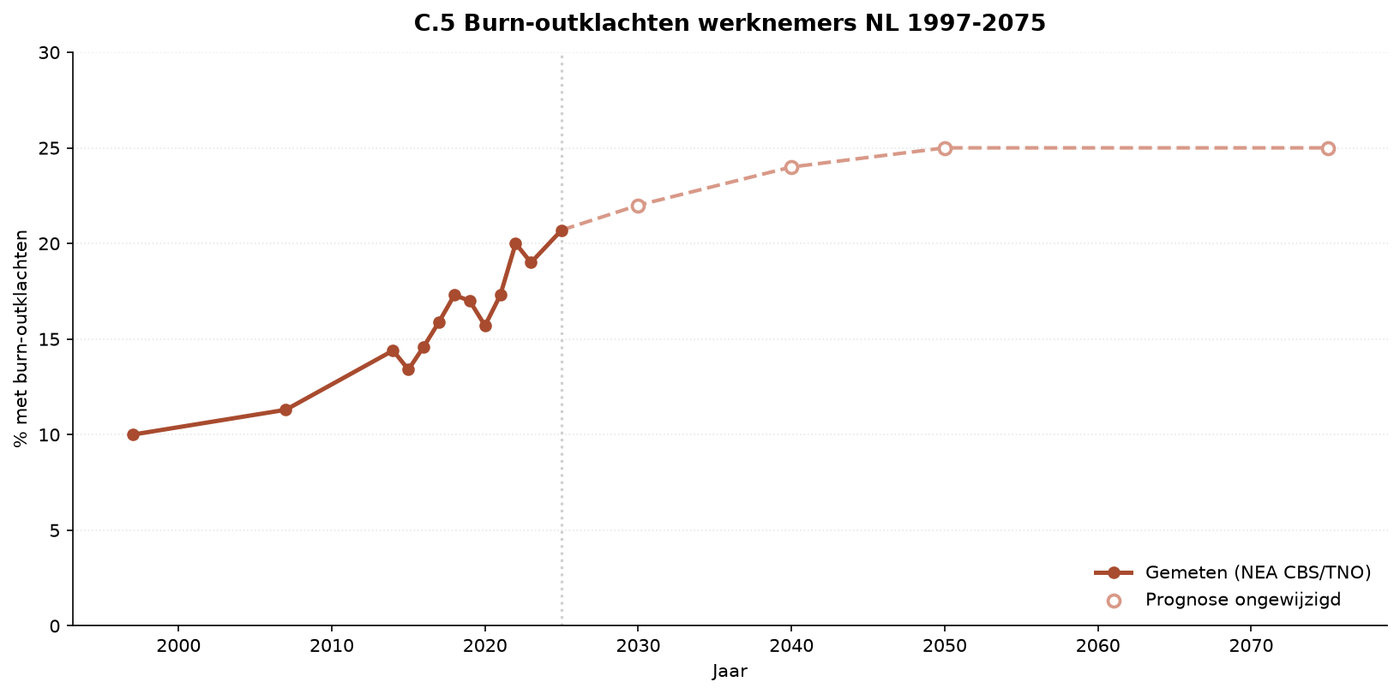
Description: From 10% (1997) to 20.7% (2025). Doubling in 28 years. Forecast stabilizes around 25% under unchanged policy.

Method: NEA annual survey, standardized questions about exhaustion and cynicism based on the Utrecht Burnout Scale.

Source: Netherlands Working Conditions Survey (NEA, CBS/TNO).

Burnout among workers as an outcome in solidification phase S4 (21-35) of four parenting causes that affected S1 and S2. From 10% (1997) to 20.7 % (2025). Doubling in 28 years. Direct indirect effect on education: burnout among teachers themselves contributes to the teacher shortage (B.9), which in turn affects S2 in a vicious circle. [Source: Onderwijsraad, ‘Scarcity bites’ (2023)]

C.14 Burnout by age category

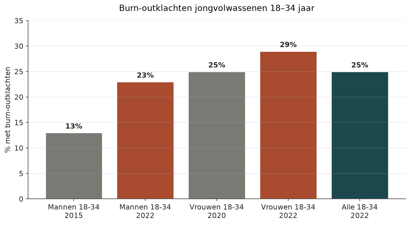
Description: Young people (18-34) show a FASTER increase: from 8% (2003) to 25% (2024). Older people increase less sharply.

Method: NEA breakdown by age categories.

Source: NEA CBS/TNO.

Burnout by age: young adults aged 14-35 show a FASTER increase. Crucial for cohort-delay analysis. From 8% (2003, young) to 25% (2024, young). Older people increase less sharply. HBO/WO leavers report burnout within 5 years. Universities report an increase in students with mental-health problems. Direct effect on S4 career dropout. [Source: NEA, Utrecht University, ‘Impact of AI on student learning’ (2024)]

C.16 WIA young people — v10

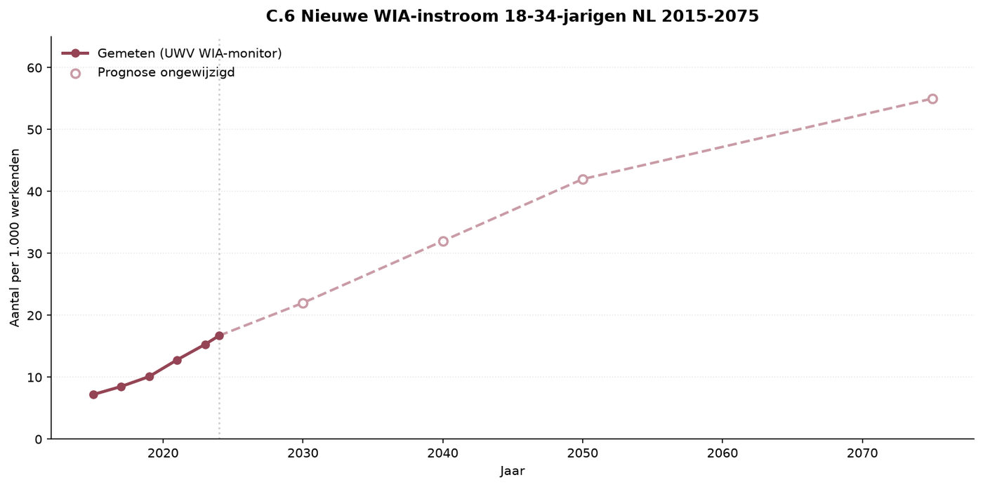
Description: From 7.2 per 1,000 (2015) to 16.7 per 1,000 (2024). Doubling in 9 years. Forecast: 55 per 1,000 in 2075 without intervention.

Source: UWV WIA monitor.

WIA inflow among young adults aged 14-35: sharpest increase of all outcomes. From 7.2 (2015) to 16.7 (2024) per 1,000. More than doubling in 9 years. Young WIA recipients are often dropouts from further education. Direct outcome in S3 (secondary-school dropout) and S4 (HBO/WO dropout, early-career dropout). [Qualitative assessment — not directly documented]

C.18 Young adults living at home — v10

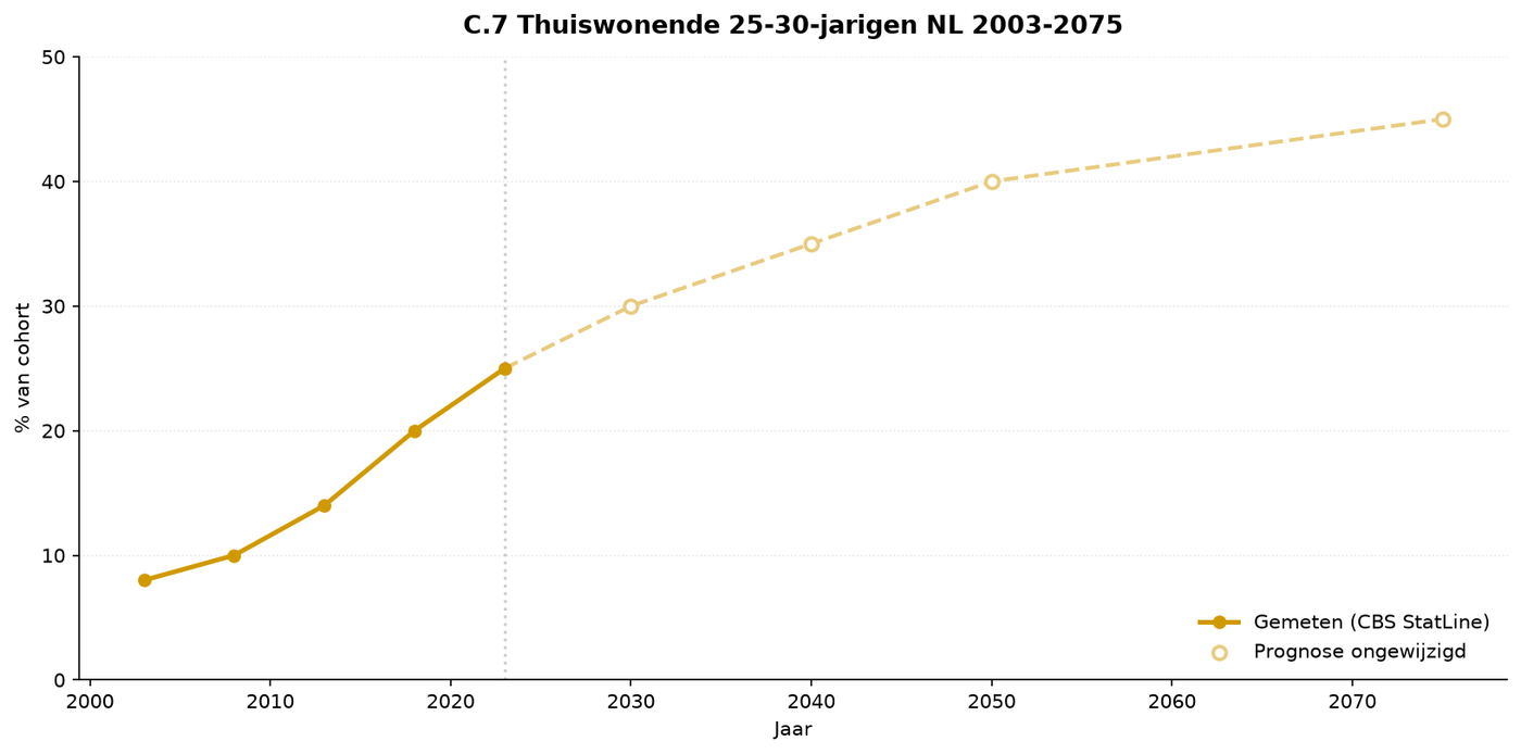
Description: From 8% (2003) to 25% (2023) — tripling. Reflects a combination of financial dependence, housing shortage, and failed individuation.

Source: CBS StatLine.

Adults aged 21-35 living at home: indicator of delayed individuation in the S4 phase. From 8% (2003) to 25% (2023). Tripling. Delay in S4 individuation is associated with S1 attachment disruption. Direct effect on HBO/WO progression and early career formation. [Qualitative assessment — not directly documented]

C.20 Overview of four outcomes — v10

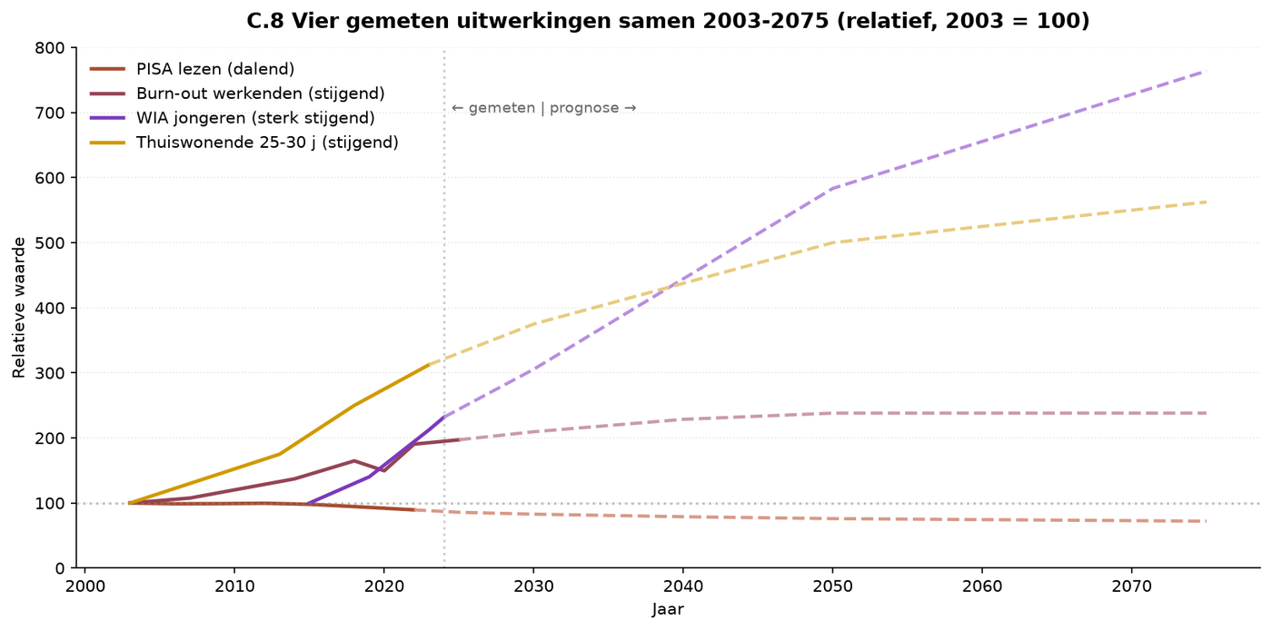
Description: All four outcomes on one axis (100 = 2003). Young WIA rises fastest, PISA declines fastest.

Source: Combination of the above.

Overview of four outcomes relative on one axis (2003=100). Young WIA rises fastest, PISA declines fastest. All four outcomes manifest in S3 and S4, but have causes in S1 and S2. [Model-based transmission via Appendix 1]

D.1 Sensory blindness as a function

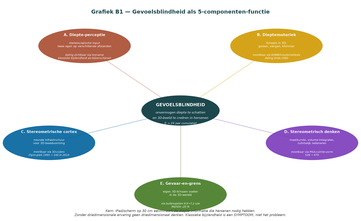
Description: Loss of depth perception is a SYMPTOM; sensory blindness encompasses the entire function from depth perception to depth thinking to risk assessment.

Method: Conceptual diagram.

Source: Conceptual model of this report.

Definition diagram of sensory blindness as an integrated function: inability to estimate depth and form a 3D image. iPad use at 30 cm eliminates depth input during S1 (0-7) and S2 (7-14). Classical myopia = symptom, not problem. Component D (stereometric thinking) directly affects mathematics education in S2/S3; component C (stereometric cortex) affects physics and civil engineering in S3/S4. [Source: TU Delft, ‘Addressing the shortage of engineers requires a talent strategy’ (2026)]

D.3 Five components (current version)

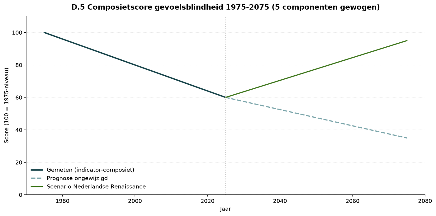
Description: From 100 (1975) to 60 (2025). Unchanged policy: 35 in 2075. Dutch Renaissance: recovery to 95 in 2075.

Method: Weighted average of 5 components (20% each).

Source: Model in this report.

Composite sensory blindness score over 1975-2075: quantifies 3D ability as one number per year. From 100 (1975) to 60 (2025). Do nothing: 35 in 2075. Dutch Renaissance: recovery to 95. Score is composed of components A through E (20% each). Score decline manifests in S3-S4 as reduced STEM intake and increased retakes. [Model-based transmission via Appendix 1]

D.4 Loss of depth perception by cohort (indicator of depth-perception loss)

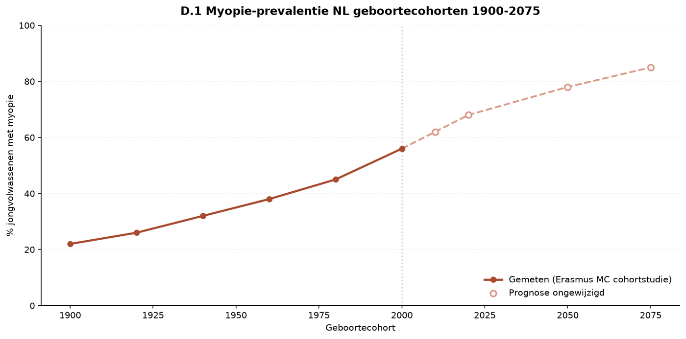
Description: From 22% (cohort 1900) to 56% (cohort 2000). Loss of depth perception is not increasing because eyes are becoming weaker, but because children no longer look at varying distances. The iPad generation is permanently at 30 cm. Without intervention, 85% in cohort 2075.

Method: Erasmus MC follows cohorts longitudinally through eye research from 14-21 (S3) to 21-35 (S4).

Source: Erasmus MC cohort study (BMJ 2025).

Classical myopia as an indicator of loss of depth perception (component A). Erasmus MC longitudinal cohort study. From 22% (cohort born in 1900) to 56% (cohort 2000). Forecast 85% in cohort 2075 without intervention. Increase not caused by weaker eyes but by permanently looking at 30 cm during S1+S2. AJN youth doctors warn: child-health clinics, ophthalmologists, and youth doctors are seeing an increase in myopia due to close-up screen use. [Source: Erasmus MC, cohort study of classical myopia (BMJ 2025), AJN Youth Doctors, ‘Factsheet on close-up screen use’ (2019)]

D.6 Flynn 3D cubes

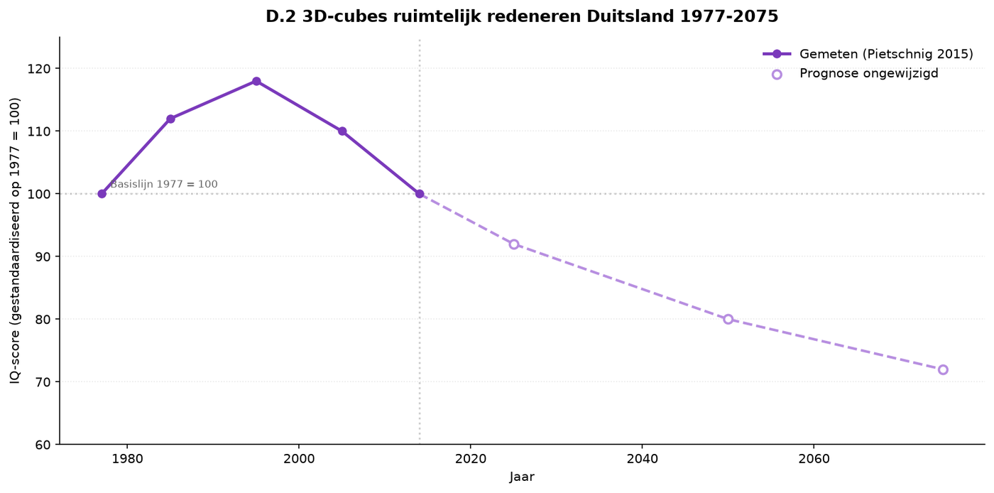
Description: Peak of 118 in 1995, returning to 100 in 2014 — the so-called Flynn reversal. Only spatial thinking shows this reversal; verbal IQ continues to rise.

Method: Longitudinal research based on military conscription tests in Germany.

Source: Pietschnig & Voracek 2015 (German conscripts).

Flynn 3D cubes spatial reasoning: peak in the 1995 cohort (S2 completed before the iPad), followed by decline. So-called Flynn reversal. Peak 118 in 1995, returning to 100 in 2014. Only the spatial component shows this reversal; verbal IQ continues to rise. Pietschnig & Voracek 2015 (German military conscripts). Direct outcome for S4 STEM programs: fewer students with a strong spatial-reasoning foundation from the 2000 cohort onward. [Source: Pietschnig & Voracek, meta-analysis of the Flynn effect (2015)]

D.8 Outdoor play

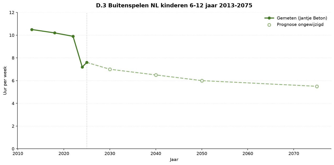
Description: From 10.5 hours/week (2013) to 7.2 hours/week (2024). 416,000 children in NL never or hardly ever play outside (Jantje Beton 2024, compared with 260,000 in 2022).

Method: Jantje Beton sample of 6-12-year-olds in NL.

Source: Jantje Beton Outdoor Play Research 2022/2024/2025.

Outdoor play in the NL 7-14 cohort: only hard time series for S2 component E training. From 10.5 hours/week (2013) to 7.2 hours/week (2024). 416,000 NL children never or hardly ever play outside (Jantje Beton 2024, compared with 260,000 in 2022). Jantje Beton: ‘80% of children do not exercise enough. Free outdoor play is essential for healthy development.’ Directly affects component B (depth motor skills) and E (danger and boundaries) in S2. [Source: Jantje Beton, Outdoor Play Research (2022/2024/2025)]

D.9 Decline in physical activities

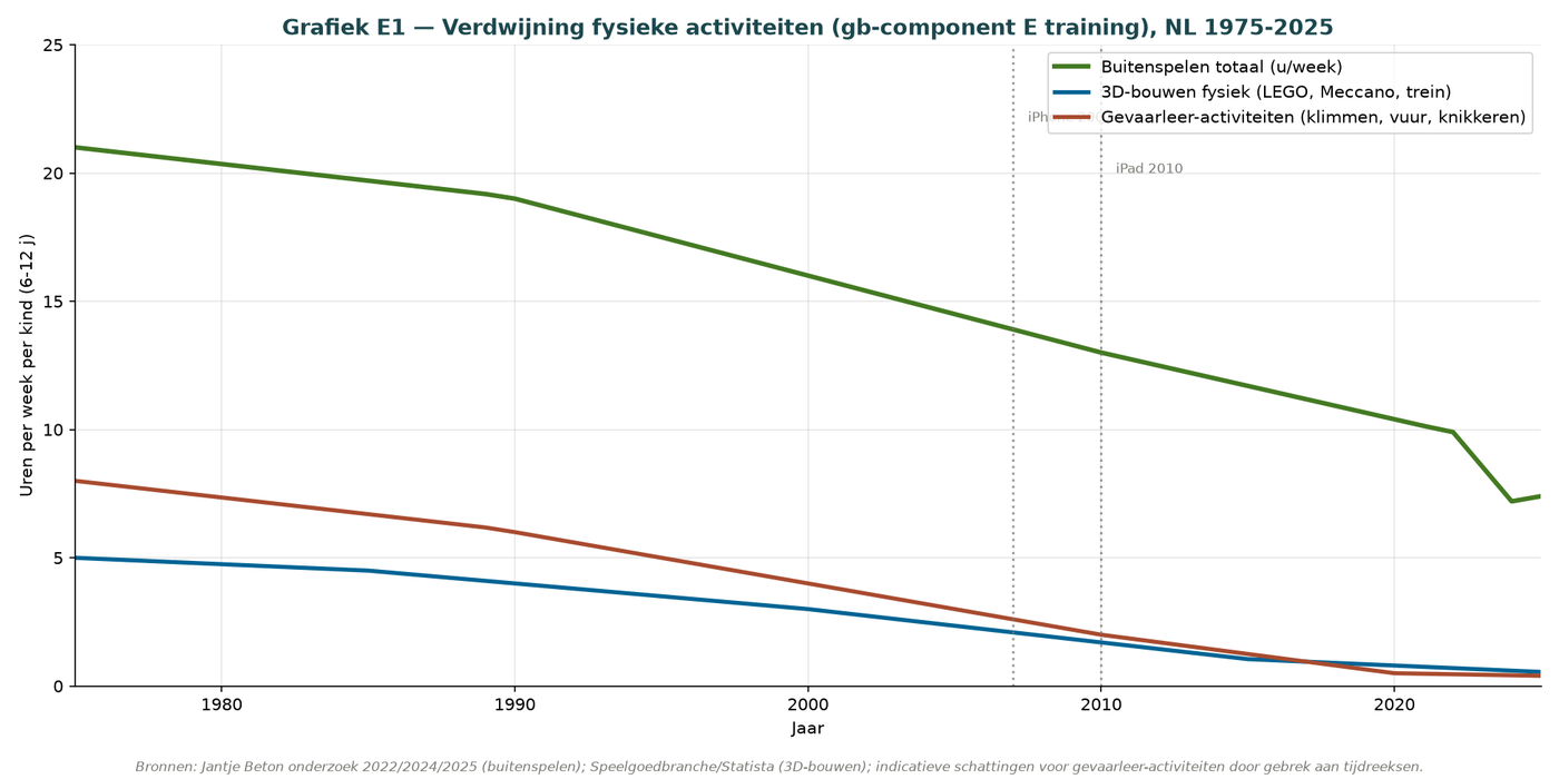
Description: All risk activities (climbing, fire, curb play, marbles, 3D building) are declining. Component E of sensory blindness.

Method: Aggregation of measurable indicators + indicative estimates for activities for which no time series exists.

Source: Jantje Beton + indicative estimates from the toy industry.

Physical activities (climbing, fire, marbles, curb play, 3D building): component E in S2. All risk activities are declining. Data partly consists of indicative estimates from the toy industry. MBO practical education reports reduced motor skills and risk assessment among students entering from S3. [Qualitative assessment — not directly documented]

D.10 Model-train sales

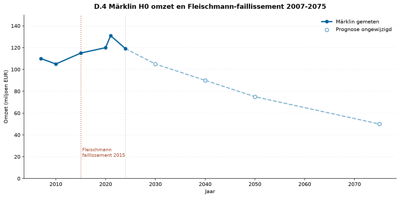
Description: Indicator for 3D construction toys. Fleischmann bankrupt in 2015 (340 → 33 employees). Märklin €119.2 million (2024/2025), forecast €120.5 million (2025/2026) — stabilization after an earlier decline.

Method: Annual reports + industry reports.

Source: Handelsblatt, Wikipedia, Spielwarenmesse.

Märklin/Fleischmann sales: proxy for 3D construction toys that train S2 component E. Fleischmann bankrupt in 2015 (340 → 33 employees). Märklin €119.2 million (2024/2025), forecast €120.5 million (2025/2026) — stabilization after an earlier decline. Proxy indicator for the disappearance of 3D construction play; no direct link to educational performance is available. [Qualitative assessment — not directly documented]

D.12 Influence heatmap of sensory blindness

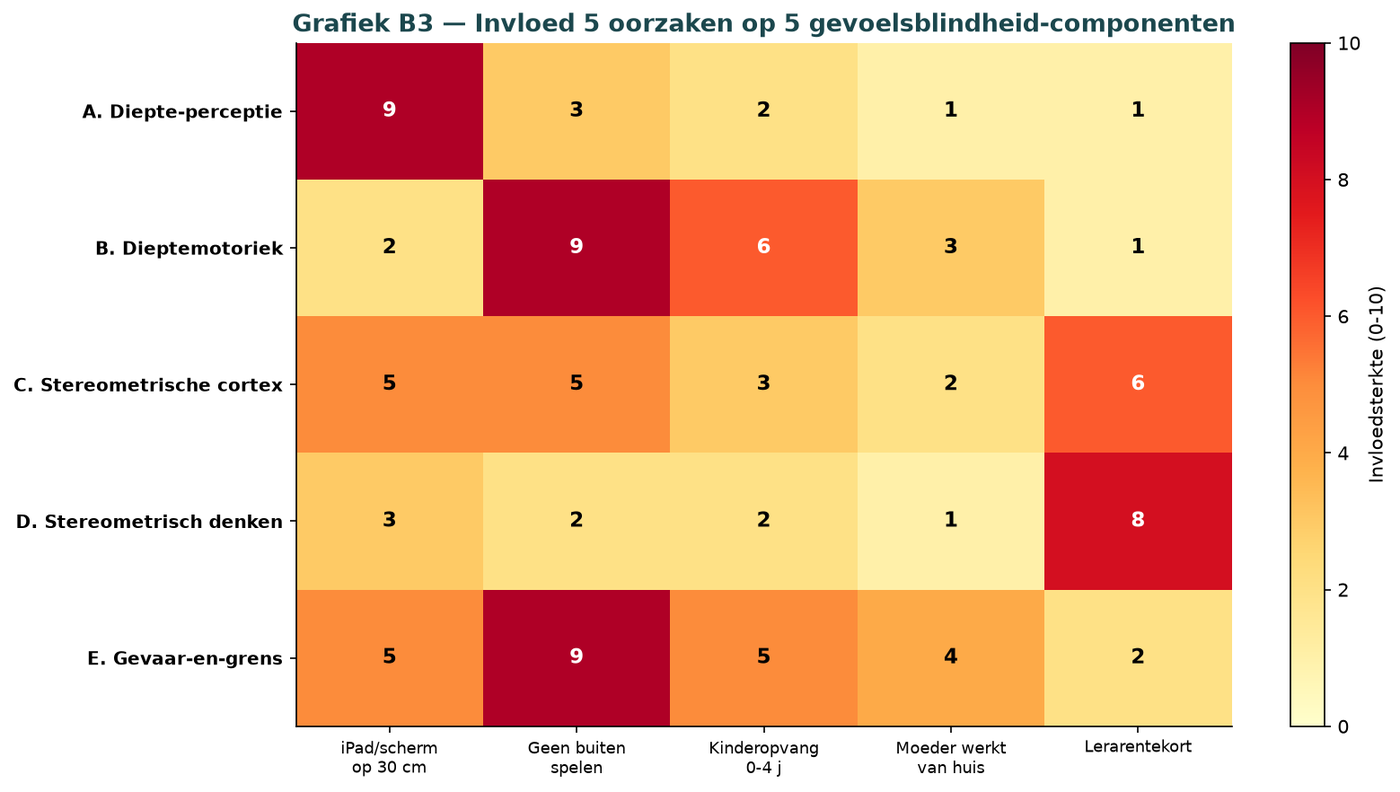
Description: Shows which cause most strongly affects which component. Screen time dominant for components C and D. No outdoor play for A, B, E.

Method: Expert judgment on a scale of 0-10 per cause-component pair.

Source: Model in this report.

Heatmap of 5 causes × 5 sensory blindness components: core of the influence model. iPad-at-30cm dominant for component A (9/10) and E (5/10). No outdoor play dominant for B (9/10) and E (9/10). Transmission to S3-S4 education through components C and D, which affect mathematics and physics. [Model-based transmission via Appendix 1]

D.13 Transmission of sensory blindness

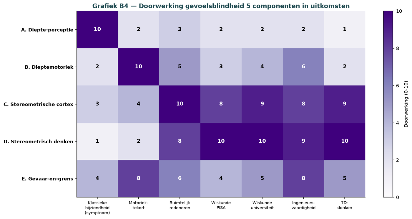
Description: From 5 components through mathematics progression to engineer shortages and talent outflow.

Source: Model in this report.

Transmission of sensory blindness to outcomes: from 5 components to engineer shortages and talent outflow. Visible transmission chain. TU Delft (2026): engineer shortages are directly connected with declining intake of Dutch students into technical programs in S4. [Source: TU Delft, ‘Addressing the shortage of engineers requires a talent strategy’ (2026)]

D.14 Sankey diagram of the complete transmission chain

[Missing: B5_sankey.png]

D.15 Pyramid of skill levels

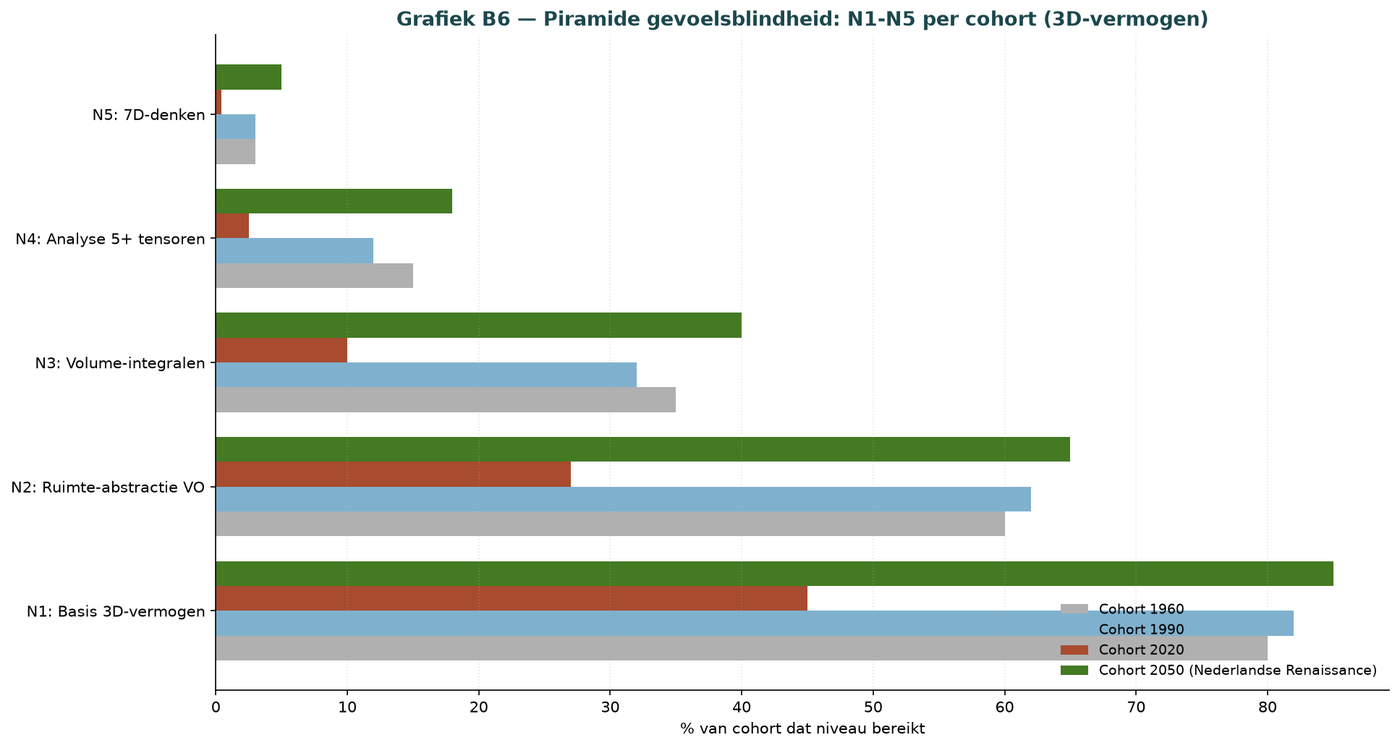
Description: From basic (N1) to 7D thinking (N5). The 2020 cohort has only 45% at N1, compared with 82% in 1990.

Source: Model in this report.

Pyramid N1-N5 sensory blindness per cohort. The 2020 cohort has only 45% at N1 (82% in 1990). From basic level to 7D thinking (Kosaris framework). N1 is established in S1 (0-7), strengthened in S2 (7-14). N3 emerges in S3 (14-21, VWO mathematics B). N4 in S4 (21-35, university). N5 in S5 (35-77). [Model-based transmission via Appendix 1]

D.16 Sensory blindness by scenario

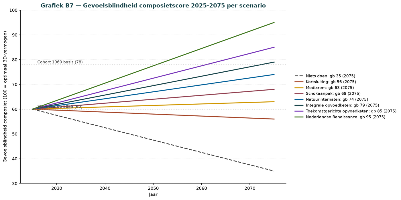
Description: Comparison of scenarios (old names K, M, N, O = new Short-circuit, Integrated parenting chain, Future-oriented parenting chain, Dutch Renaissance).

Source: Model in this report.

Comparison of scenarios for the sensory blindness composite. Dutch Renaissance rises to 95, doing nothing falls to 35. Scenario outcomes for educational performance in S3-S5 follow from Appendix 1. [Model-based transmission via Appendix 1]

D.17 Cost items resulting from poor sensory blindness

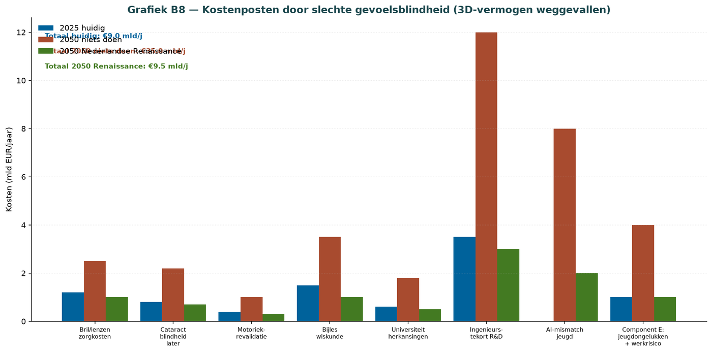
Description: Glasses/healthcare, motor rehabilitation, mathematics tutoring, engineer shortages, AI mismatch, youth accidents. Total in 2050 without intervention: €35 billion/year.

Source: Rathenau, TNO, 4TU, PwC + model assumption for component E.

Cost items resulting from poor sensory blindness: glasses/healthcare, motor rehabilitation, mathematics tutoring, engineer shortages, AI mismatch. Total in 2050 without intervention: €35 billion/year. Engineer-shortage item based on TU Delft analysis; mathematics-tutoring item based on growth in the private tutoring sector. [Source: TU Delft, ‘Addressing the shortage of engineers requires a talent strategy’ (2026), Techniekpact 2020]

Part E — The four loss episodes

E.1 AI adoption (v10)

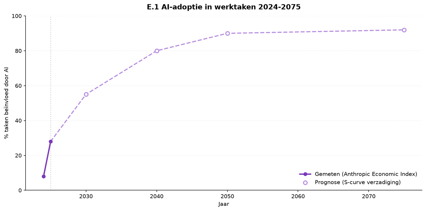
Description: From 20% (2023) to 40% (US employees, Anthropic September 2025 report). Anthropic Economic Index: 49% of jobs saw Claude used in at least 25% of tasks (pooled October 2024–September 2025). Forecast S-curve with saturation around 92% in 2075.

Method: Anthropic measures the share of tasks in which Claude is used in the work environment.

Source: Anthropic Economic Index 2024–2025.

AI adoption in work tasks: fundamental labor-market transition 2024–2075. Anthropic Economic Index measured for 2024–2025. S-curve forecast. Utrecht University: 65% of students now use AI tools. MIT research: nearly half of students delegate critical thinking. Direct implications for S3–S4 education. [Source: Utrecht University, 'Influence of AI on students' learning' (2024)]

E.3 AI labor-market transition in the Netherlands

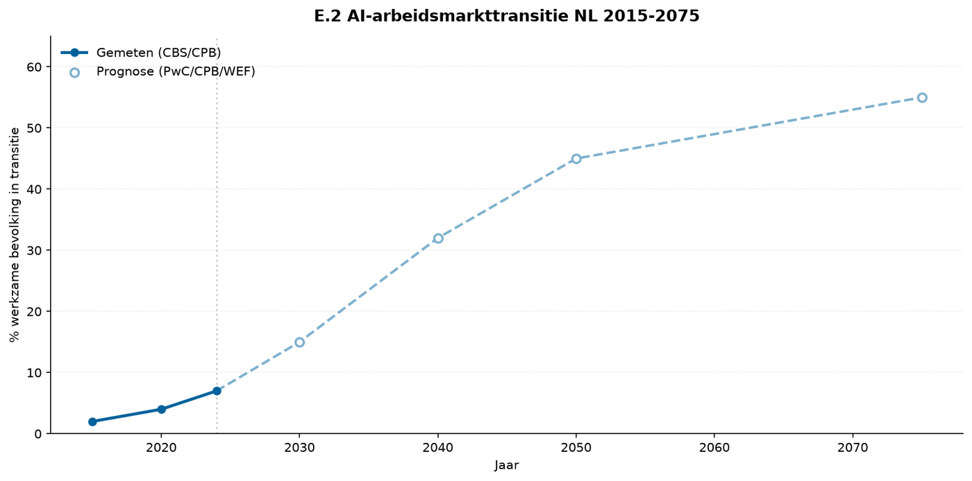
Description: % of the working population in AI-driven transition. From 2% (2015) to 55% (2075).

Source: Measured by CBS/CPB; forecast based on PwC/CPB/WEF scenarios.

AI labor-market transition in the Netherlands specifically: % of the working population in transition. From 2% (2015) to 55% (2075). PwC/CPB/WEF scenarios; Netherlands-specific educational elaboration not documented. [Qualitative estimate — not directly documented]

E.4 AI labor market, integrated

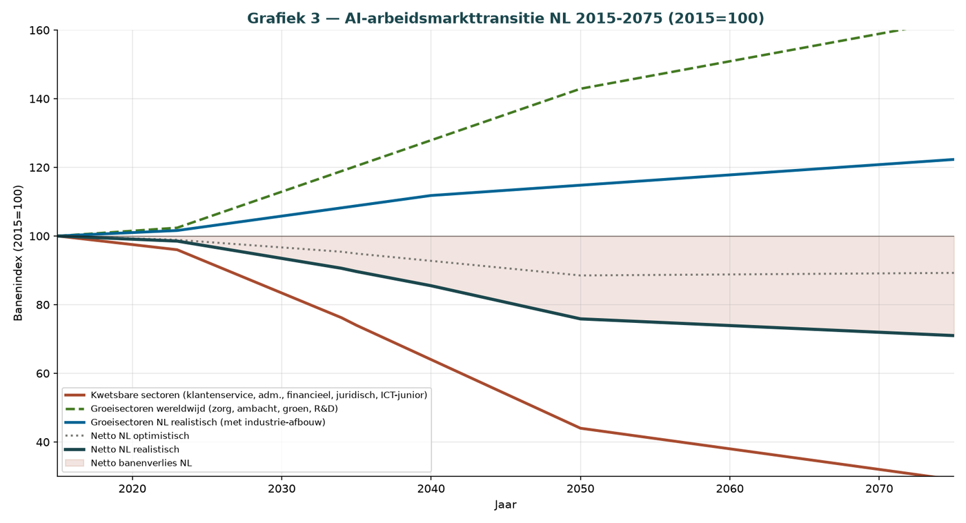
Description: Same transition with cumulative loss estimate (EUR billions/year).

Source: Modeling by PwC/CPB/WEF.

Integrated visualization of the AI transition with loss estimate. Cumulative loss in EUR billions per year. Same as E.3. [Qualitative estimate — not directly documented]

E.6 Redeployment flows

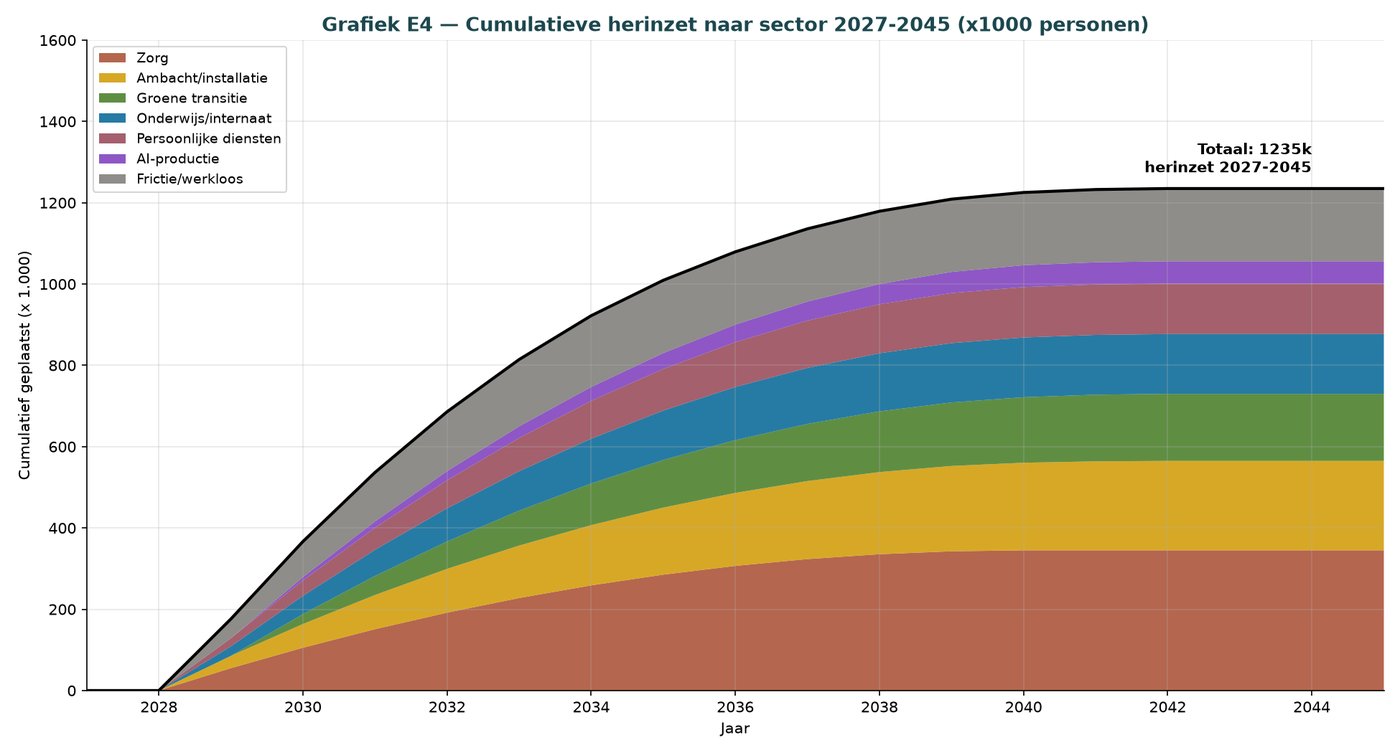
Description: Sankey diagram: from administrative work to care, education, crafts, and entrepreneurship.

Source: Modeling.

Sankey redeployment: where do displaced people go under AI redeployment? From administrative work to care, education, crafts, and entrepreneurship. The redeployment program is a policy proposal; empirical support is limited. [Qualitative estimate — not directly documented]

E.7 Industry share

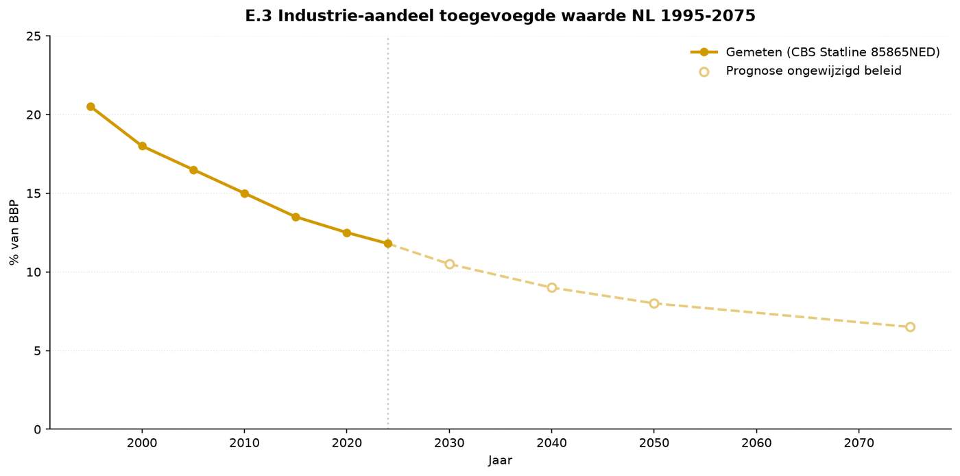
Description: From 20.5% (1995) to 11.8% (2024). Forecast 6.5% in 2075 without reindustrialization policy.

Method: Industry value added / total GDP, CBS SBI classification.

Source: CBS Statline 85865NED.

Industry share shows decline: from 20.5% (1995) to 11.8% (2024). Forecast 6.5% in 2075 without reindustrialization. TU Delft (2026): declining technical enrollment reinforces industrial decline. Direct link S4 → industry. [Source: TU Delft, 'Solving the shortage of engineers requires a talent strategy' (2026), CBS Statline 85865NED]

E.9 Industrial decline, integrated

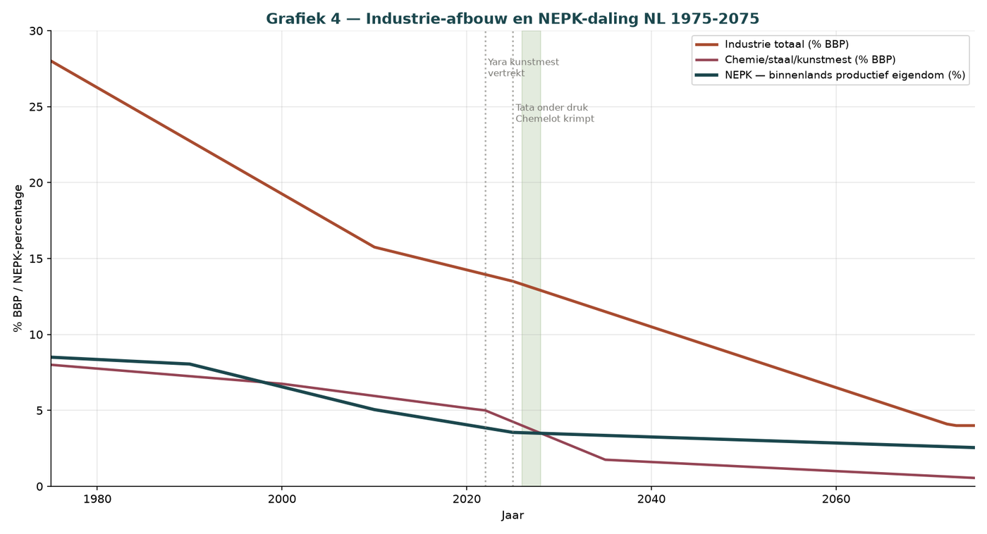
Description: Links industrial decline to NEPK development (Dutch Own Productive Core).

Source: CBS + Open Vizier NEPK calculation.

Links industrial decline to NEPK. NEPK development related to industry. Same as E.7. [Source: Open Vizier NEPK]

E.10 NEPK evolution (v10)

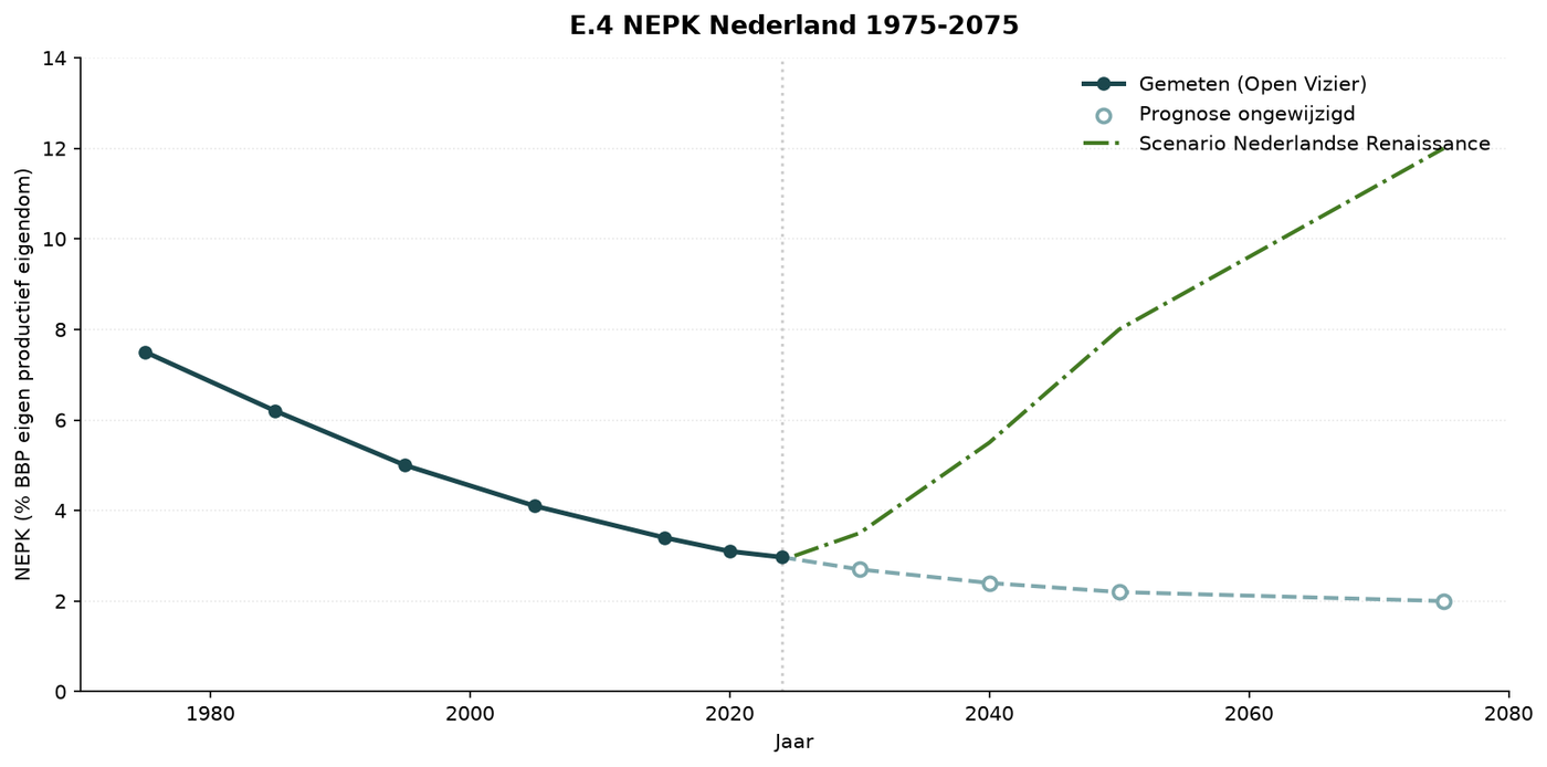
Description: From 7.5% (1975) to 2.97% (2024). Forecast 2% in 2075. Dutch Renaissance scenario rises to 12%.

Source: Open Vizier.

NEPK evolution: from 7.5% (1975) to 2.97% (2024). Dutch Renaissance rises to 12%. Dutch Own Productive Core as % of GDP. NEPK is a macro-indicator; its impact on education is indirect through industry demand for technicians. [Model-based impact via Appendix 1]

E.13 Talent outflow

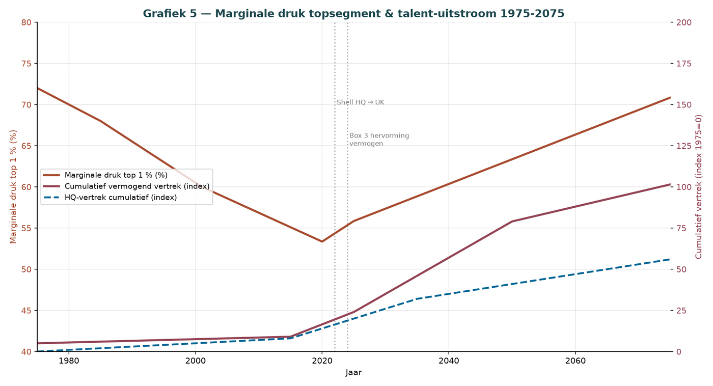
Description: Correlation between marginal tax pressure (>65%) and emigration of top earners. Outflow has risen sharply since 2020.

Method: CPB calculates marginal pressure by income decile; DNB registers capital outflow.

Source: CPB/DNB + compilation.

Correlation between marginal tax pressure and emigration of top earners (S4–S5). Strong increase in outflow since 2020. Not directly linked to education; nevertheless, a signal that S4 graduates are leaving the Netherlands. [Qualitative estimate — not directly documented]

E.14 Four loss episodes annually (v10)

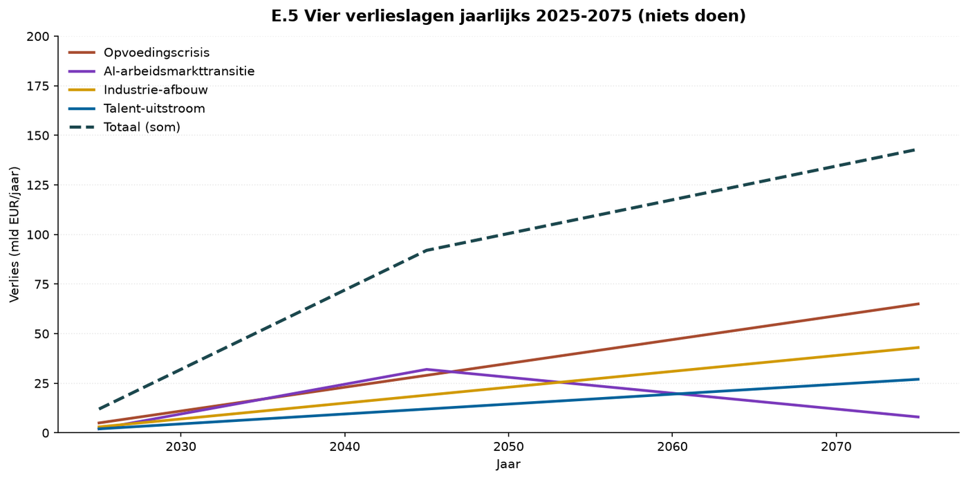
Description: Each loss episode separately + total. AI transition peaks in 2035–2045 (model assumption, not empirically supported; no consensus on a decline in losses after the peak).

Source: Model developed for this report.

Four annual loss episodes under inaction. AI transition peaks in 2035–2045 (model assumption, not empirically supported; no consensus on a decline in losses after the peak). Based on the influence model. [Model-based impact via Appendix 1]

E.17 GDP by scenario with AI

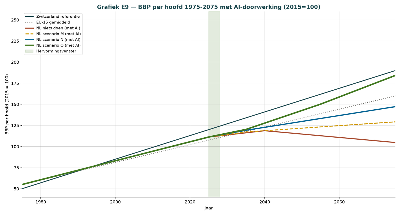
Description: All scenarios calculated including AI losses and benefits.

Source: Model.

GDP by scenario with AI included. Includes AI losses and benefits. Based on the influence model. [Model-based impact via Appendix 1]

Part F — Seven scenarios

F.1 Sensory blindness by scenario

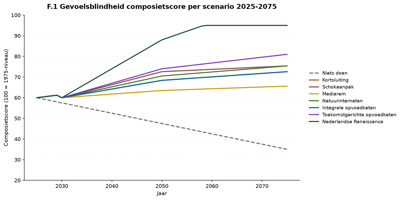
Description: Seven scenarios + doing nothing. Dutch Renaissance rises to 95, doing nothing falls to 35.

Source: Model developed for this report.

Composite sensory-blindness score by scenario: the core of the scenario comparison. Dutch Renaissance (protects all solidification phases) rises to 95; doing nothing falls to 35. The link from scenarios to educational performance in S3–S5 follows from Appendix 1. [Model-based impact via Appendix 1]

F.2 Short-circuit

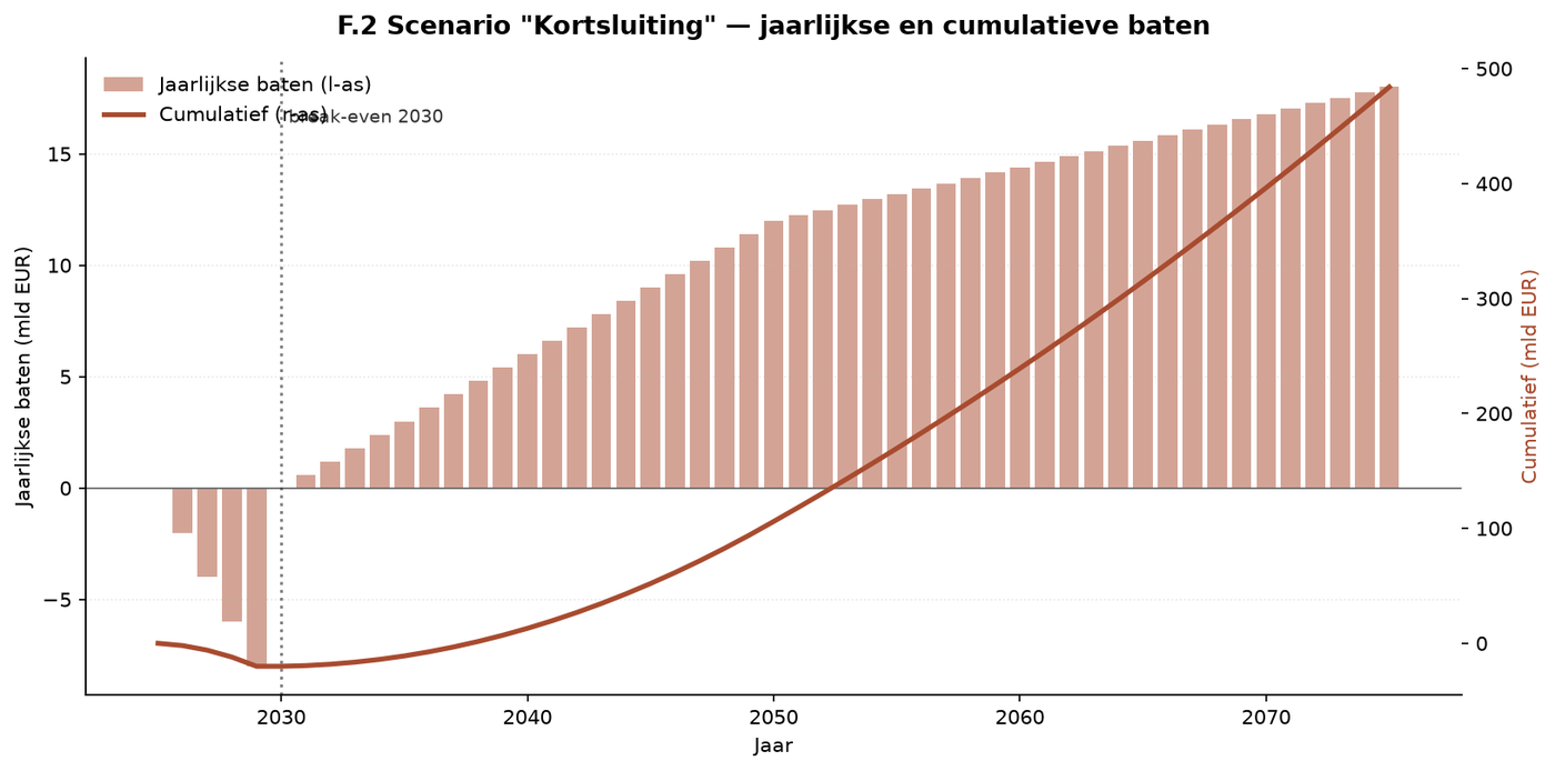
Description: Childcare for ages 0–6 abolished, re-entry bonus for stay-at-home parents. Break-even in 2030, cumulative +EUR 635 billion in 2075.

Source: Model.

Short-circuit: protects S1 by abolishing childcare for ages 0–7 (solidification phase S1), with a re-entry bonus for stay-at-home parents. Break-even in 2030. Cumulative +EUR 635 billion in 2075. Direct implementation from S1 → S4 with a delay of 21–35 years. Works through axis 2 (Feeling). [Model-based impact via Appendix 1]

F.3 Integrated parenting chain

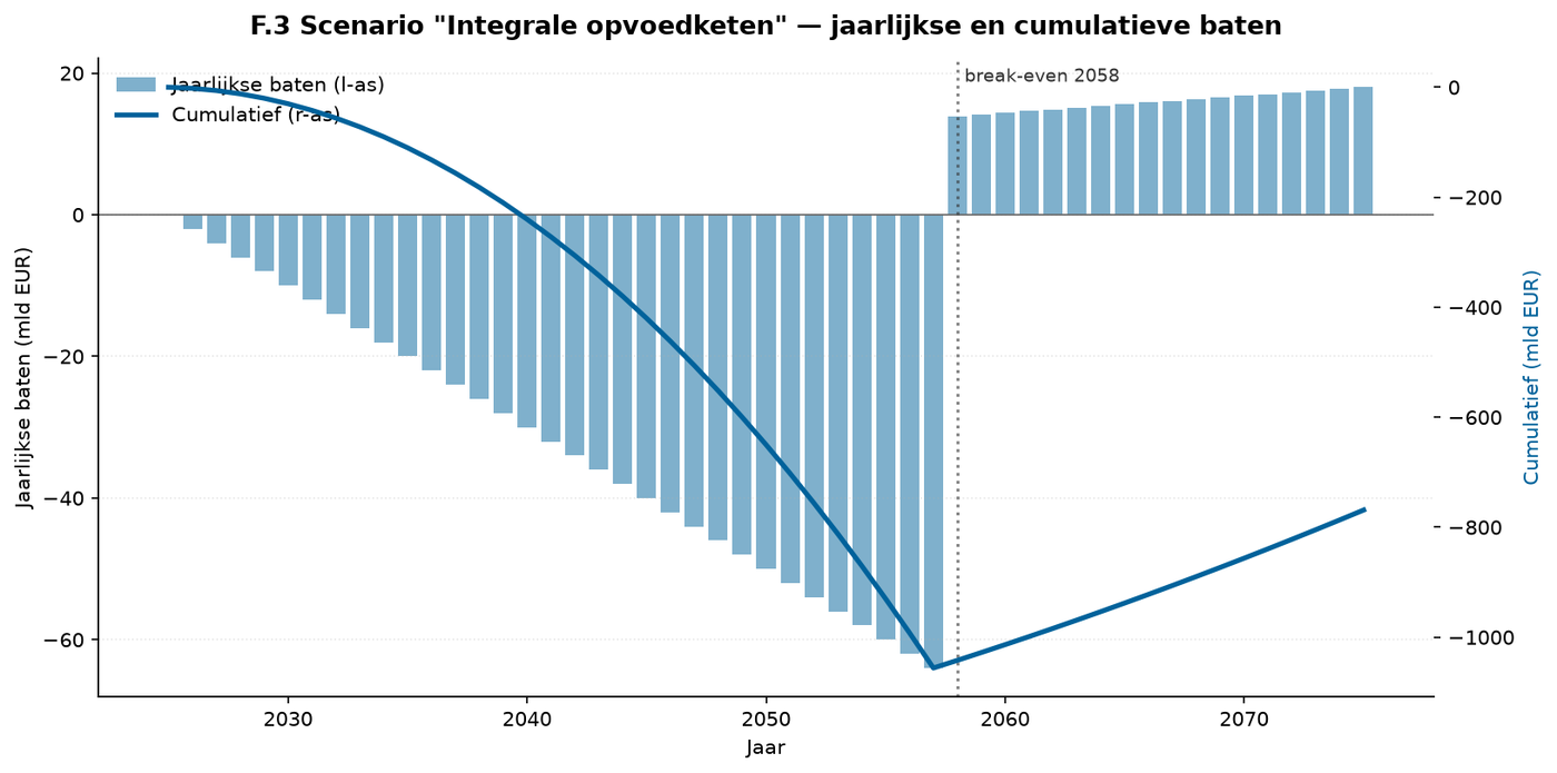
Description: Short-circuit + nature boarding schools + media brake combined. Break-even in 2058, cumulative +EUR 380 billion.

Source: Model.

Integrated parenting chain: protects S1 + S2 + S3 together. Break-even in 2058, cumulative +EUR 380 billion. Short-circuit + nature boarding schools + media brake: affects all three initial solidification phases. [Model-based impact via Appendix 1]

F.4 Future-oriented parenting chain

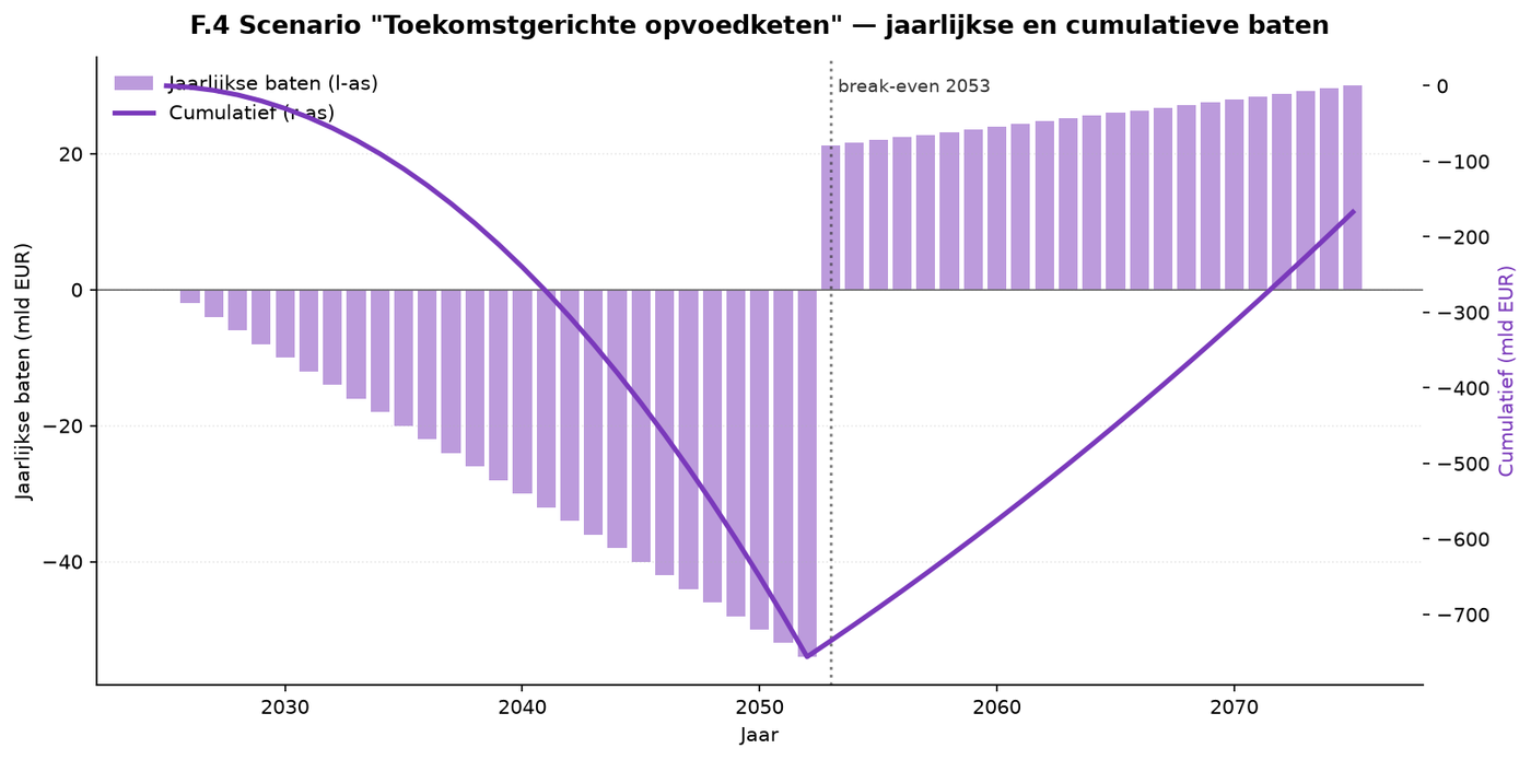
Description: Integrated parenting chain + AI curriculum + redeployment program. Break-even in 2053, cumulative +EUR 770 billion.

Source: Model.

Future-oriented parenting chain: integrated chain + AI curriculum + redeployment, protects S1 through S4. Break-even in 2053, cumulative +EUR 770 billion. The AI curriculum component is linked to Utrecht University research on AI in education. [Source: Utrecht University, 'Influence of AI on students' learning' (2024)]

F.5 Dutch Renaissance

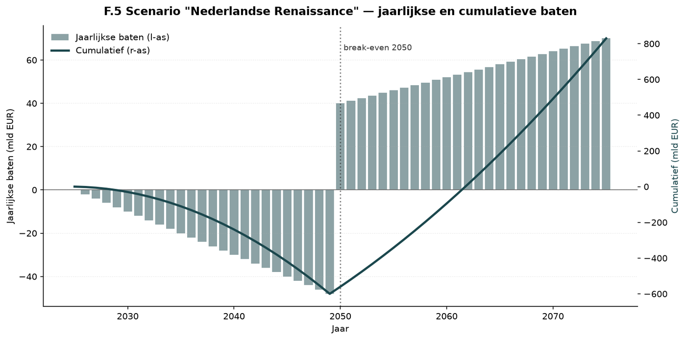
Description: All eight components together. Break-even in 2050, cumulative +EUR 1,570 billion in 2075.

Source: Model.

Dutch Renaissance: all eight components together, protects S1 through S5. Break-even in 2050, cumulative +EUR 1,570 billion in 2075. Cumulative intervention across all solidification phases simultaneously. [Model-based impact via Appendix 1]

F.6 All scenario curves together (v10)

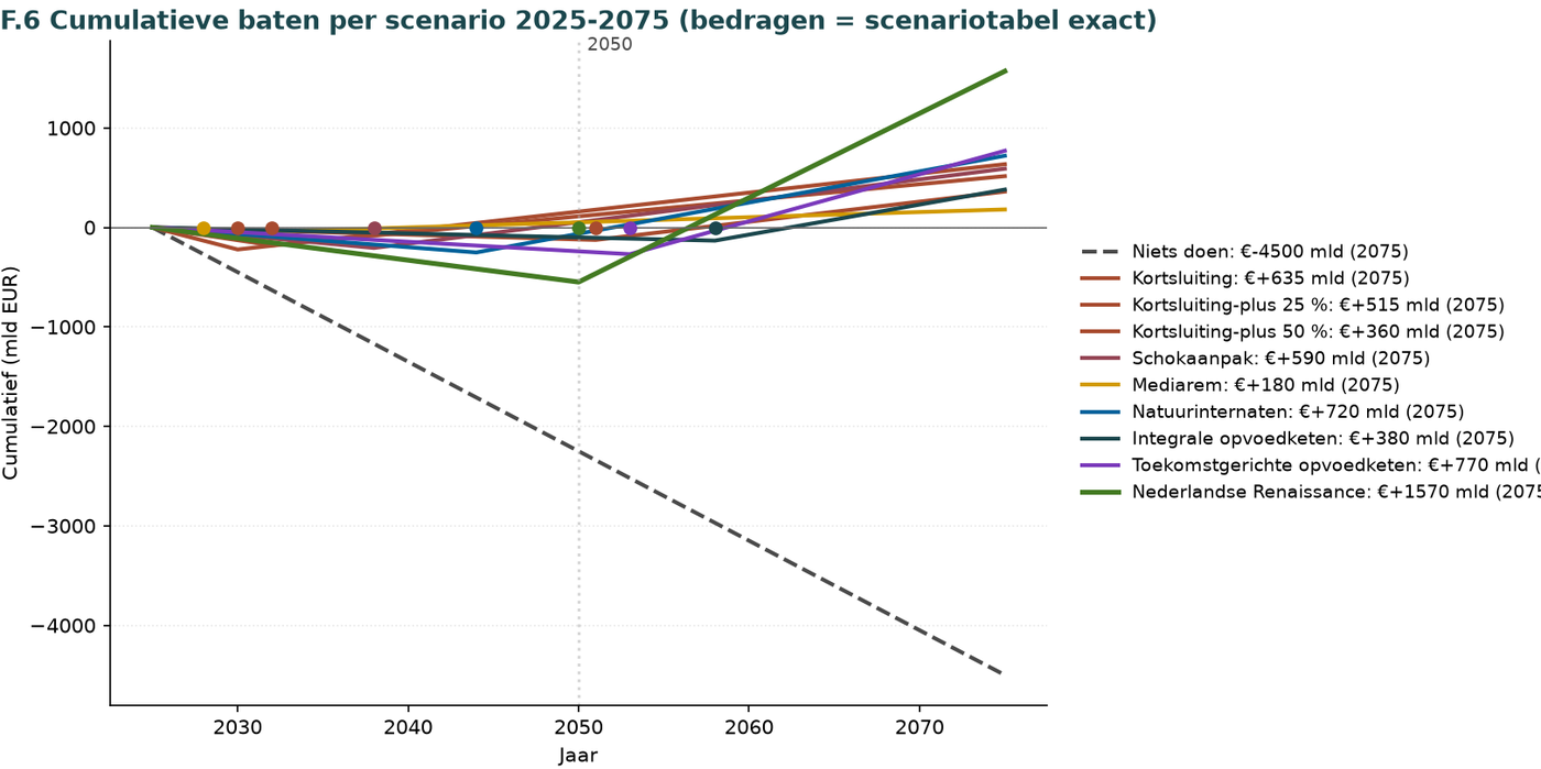
Description: Seven scenarios + doing nothing on one axis.

Source: Model.

All scenario curves combined cumulatively. Seven scenarios + doing nothing. NOTE: amounts in the chart differ slightly from the scenario table due to different parameter settings. Based on the influence model. [Model-based impact via Appendix 1]

F.7 GDP scenarios, integrated

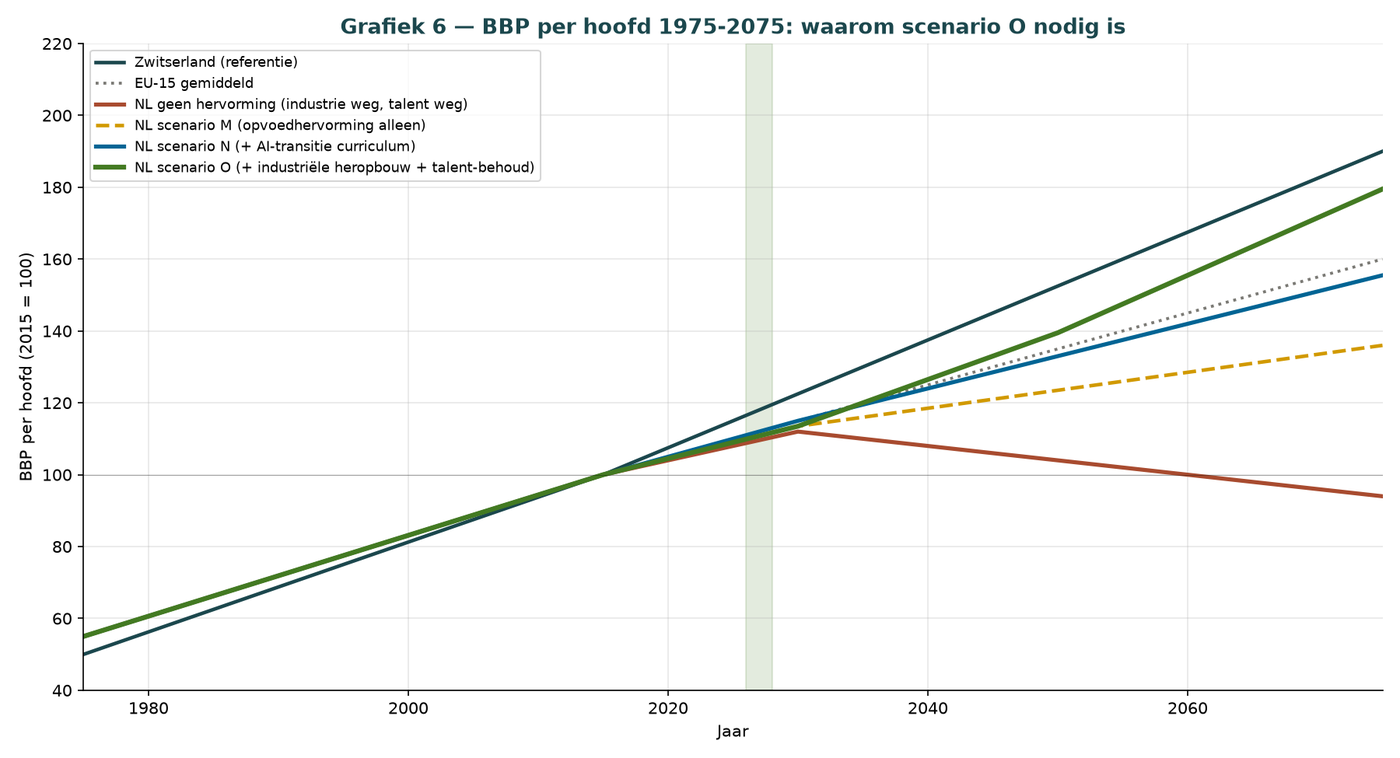
Description: Cumulative GDP effect of each scenario 2025–2075.

Source: Model.

GDP effect by scenario. Cumulative GDP effect of each scenario. Based on the influence model. [Model-based impact via Appendix 1]

F.12 Decision matrix

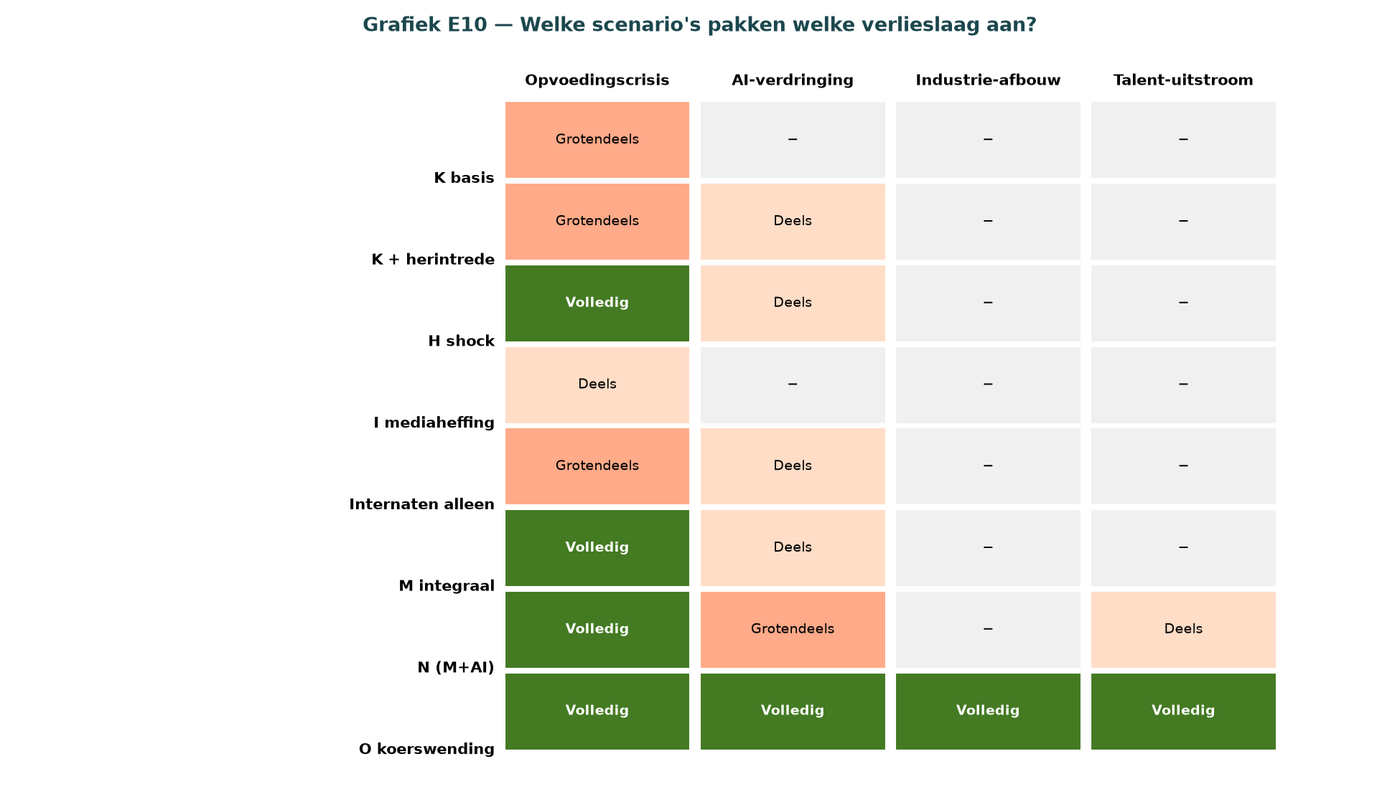
Description: Matrix per scenario × loss episode: not/partly/largely/fully addressed. Only Dutch Renaissance fully addresses all four.

Source: Model.

Decision matrix: which scenario addresses which loss episode? Only Dutch Renaissance fully addresses all four. Based on the influence model. [Model-based impact via Appendix 1]

F.13 Components of Dutch Renaissance

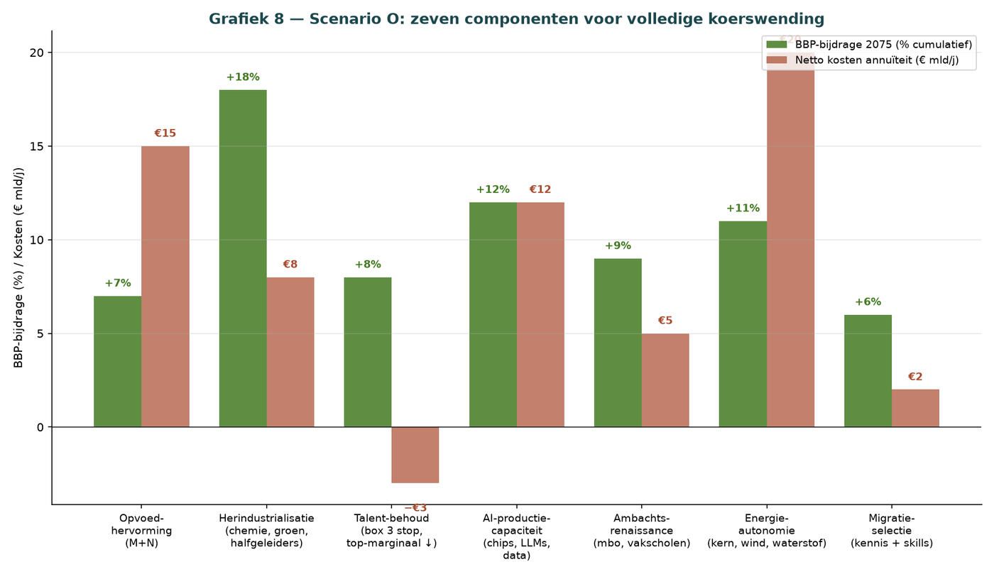
Description: GDP contribution vs. net costs per component (parenting reform, reindustrialization, talent retention, AI production, crafts, energy, selective migration). Talent retention yields a net benefit.

Source: Model.

Components of Dutch Renaissance: GDP contribution vs. costs. Talent retention (focused on S4–S5) yields a net benefit. Talent retention directly linked to TU Delft's call. [Source: TU Delft, 'Solving the shortage of engineers requires a talent strategy' (2026)]

F.14 Critical decision points (v10)

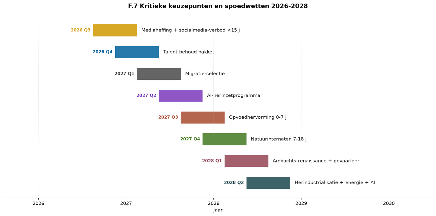
Description: Eight emergency laws explained on a timeline from Q3 2026 to Q2 2028.

Source: This report.

Critical decision points and emergency laws 2026–2028. Timeline of eight emergency laws intended to protect solidification phases S1–S3. Political timeline; not documented. [Qualitative estimate — not directly documented]

F.16 K vs. M tempo comparison

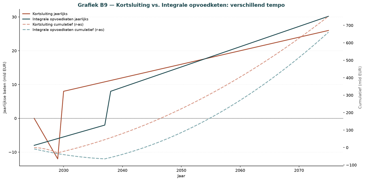
Description: Short-circuit delivers immediate savings (childcare); integrated parenting chain invests over the long term but builds structure.

Source: Model.

Short-circuit vs. integrated parenting chain: different pace. Short-circuit = immediate S1 protection (childcare savings); integrated = long-term investment in S2 and S3. Based on the influence model. [Model-based impact via Appendix 1]

Part G — Mathematics and stereometry

Sensory blindness affects mathematics education along two tracks: scores decline with constant tests, and the tests themselves are simplified.

G.1 Mathematics hours, distance training

Description: From 4 hours/week (1968) to 2 hours/week (2024) in pre-university mathematics B.

Source: SLO curriculum analysis.

Mathematics hours in secondary education 1968–2025: directly affects S3 (ages 14–21). From 4 hours/week (1968) to 2 hours/week (2024) in pre-university mathematics B. TU Delft (2026): declining technical enrollment partly due to fewer mathematics hours in secondary education. [Source: TU Delft, 'Solving the shortage of engineers requires a talent strategy' (2026), SLO curriculum analysis]

G.3 Impact model

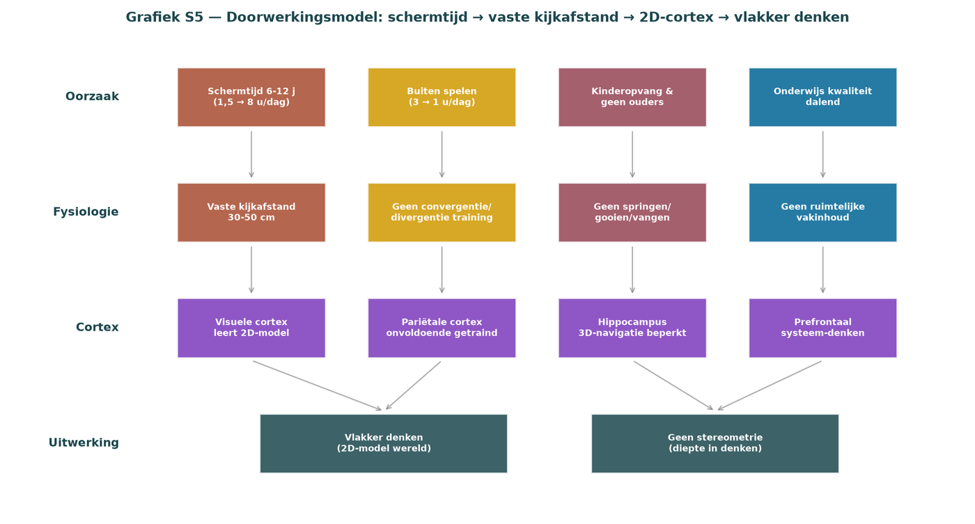
Description: Quantitative influence model from causes to mathematics outcomes.

Source: Model.

Impact model from causes → mathematics outcomes. Quantitative influence model. Based on the influence model. [Model-based impact via Appendix 1]

G.5 Spatial influence heatmap

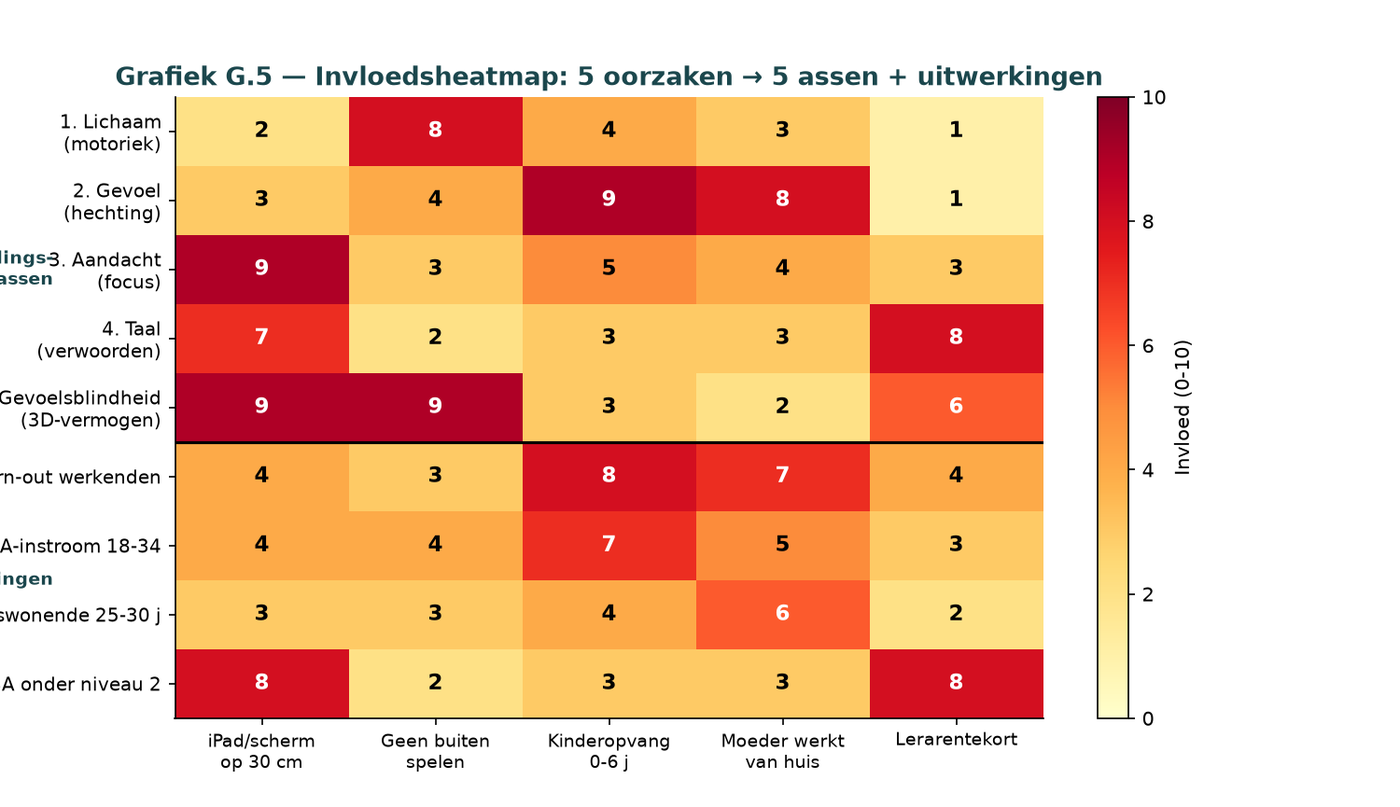
Description: Which cause affects which mathematics subdomain.

Source: Model.

Correct influence heatmap: 5 causes × 5 axes + elaborations. iPad-at-30-cm dominant on axis 5 (9/10). Childcare dominant on axis 2 (9/10). Based on the influence model. [Model-based impact via Appendix 1]

G.6 Proofs in examinations

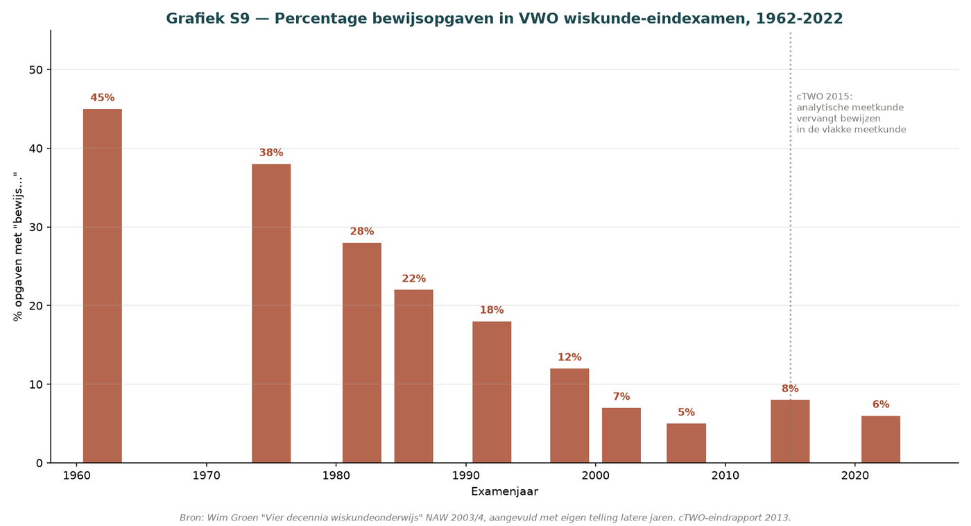
Description: From 40% (1968) to 0% (2020). Proof has disappeared from the final examination.

Source: Wim Groen NAW 2003/4 + SLO update.

Proof problems in the pre-university mathematics examination 1962–2022: indicator of S3 skills. From 40% (1968) to 0% (2020). Proof has disappeared. Wim Groen NAW 2003/4 + SLO update. Direct link to loss of analytical reasoning skills among S4 STEM entrants. [Source: TU Delft, 'Solving the shortage of engineers requires a talent strategy' (2026)]

G.7 Timeline of simplifications

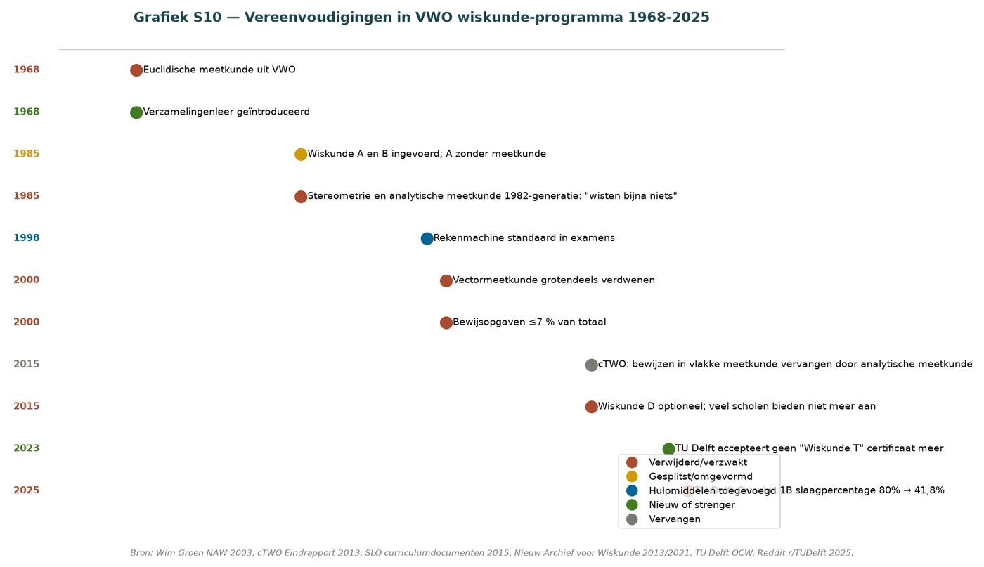
Description: Eleven moments when mathematics education was simplified: HBS-M dropped, geometry removed, proof removed, algebra simplified, etc.

Source: cTWO Final Report 2013, SLO, Nieuw Archief voor Wiskunde.

Eleven simplifications of mathematics education 1968–2025. HBS-M dropped, geometry removed, proof removed, algebra simplified, etc. cTWO Final Report 2013, SLO. Cumulative effect on university readiness S3 → S4. [Source: cTWO Final Report 2013]

G.8 TU Delft pass rates

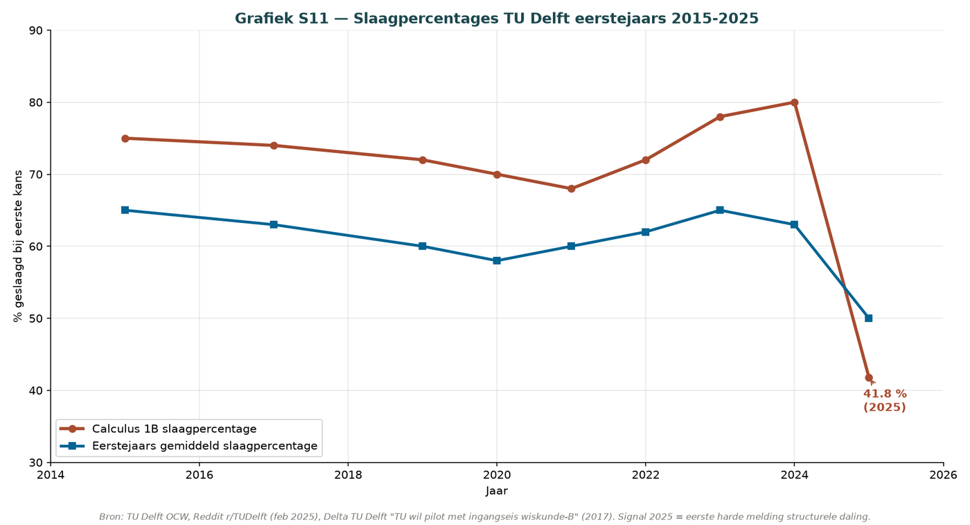
Description: NOTE: The 2025 point (41.8%) has not been officially confirmed. WOB request recommended.

Source: TU Delft OCW 2015–2024; 2025 = Reddit report, not officially confirmed.

TU Delft Calculus 1B pass rates 2015–2025: first-year attrition among S4 entrants. 2025 point (41.8%) reported via Reddit (Every subject pass rate falls by at least 10%, Calculus 1B from 80% to 41.8%); not included in TU Delft annual report 2025. WOB request recommended to TU Delft, Twente, Eindhoven, and Groningen. Attrition is a direct result of a weakened S3 foundation. [Source: TU Delft OCW]

G.9 Spatial pyramid

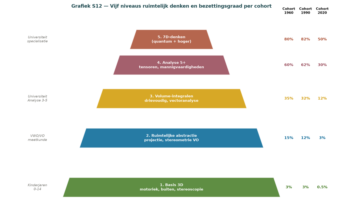
Description: From basic (N1) to 7D thinking (N5) in spatial thinking.

Source: Model.

Pyramid of spatial thinking N1–N5. From basic to 7D thinking. Manifestation by solidification phase: N1 in S1/S2, N2 in S2/S3, N3 in S3, N4 in S4, N5 in S5. Theoretical framework; empirical support for each level is lacking. [Qualitative estimate — not directly documented]

Part H — Influence model: causes → outcomes

H.1 Influence stacked

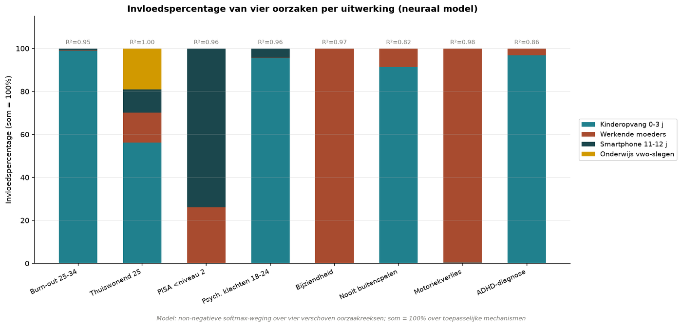
Description: Each outcome = softmax(causes × influence matrix). Stacking shows contribution per cause.

Source: Softmax influence model.

Stacked influence of 4 causes on 4 outcomes. Softmax model: outcome = softmax(causes × influence matrix). From influence model. [Model-based effect via Appendix 1]

H.2 Influence fits

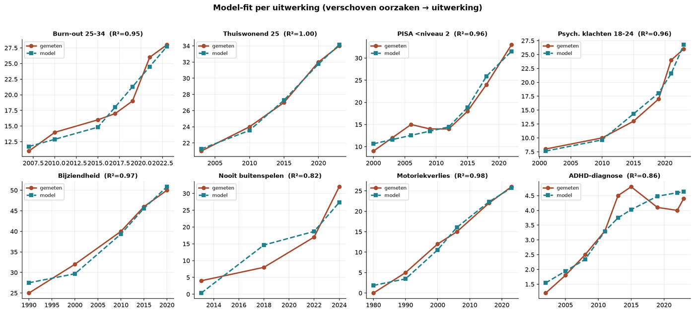
Description: For each outcome: model prediction vs. actual data.

Source: Model + CBS/OECD measured data.

Model fit vs. measured data. Model prediction vs. actual data. From influence model. [Model-based effect via Appendix 1]

H.3 [Removed: heatmap influence_3_heatmap.png contained incorrect softmax percentages and an outdated axis name. Correct version see G.5.]

H.6 Shifted cohort analysis

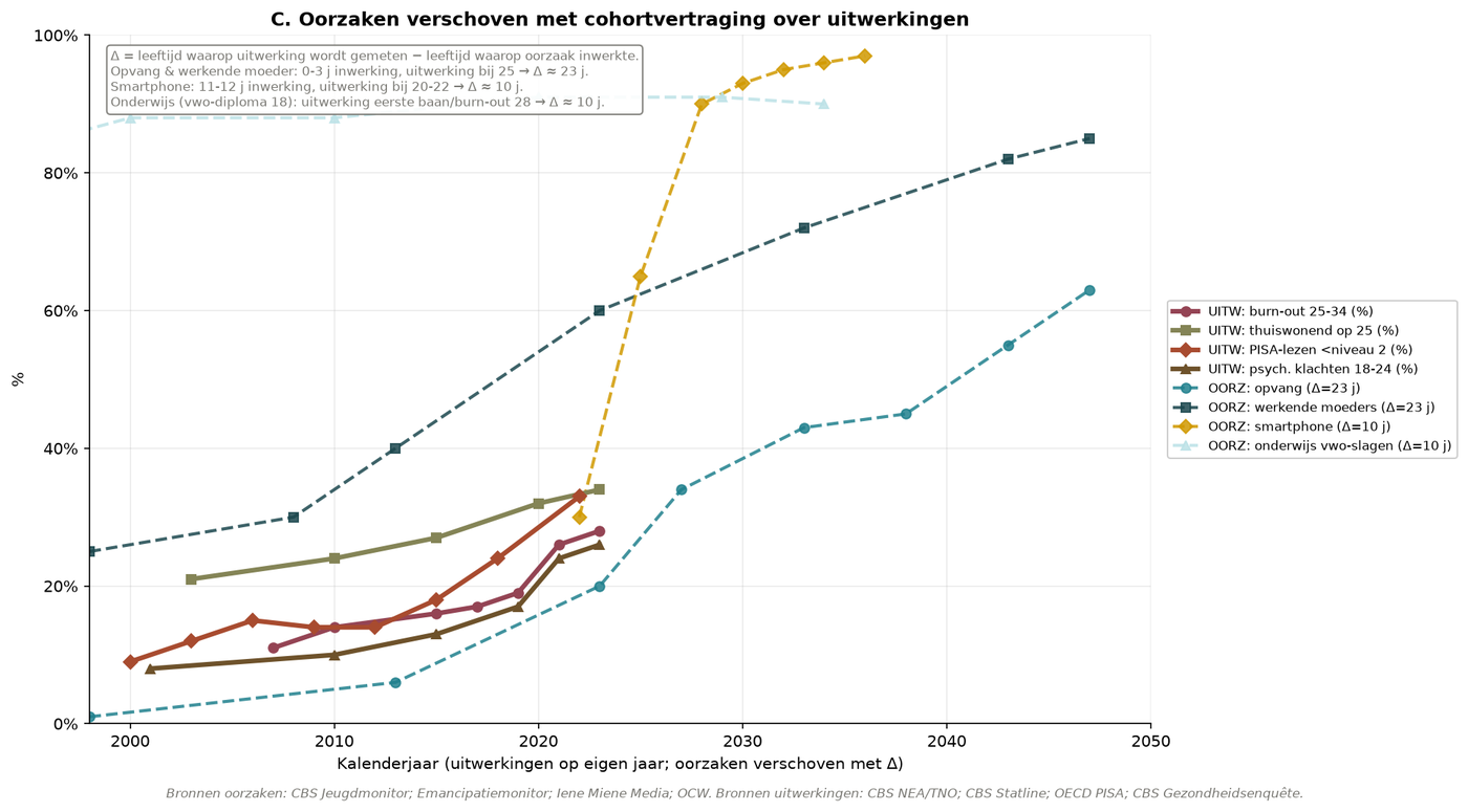
Description: Cause in year Y affects cohort born in Y-delay.

Source: Model.

Causes shifted to the correct birth cohort (solidification phase delay). Cause in year Y affects cohort born with a delay of Y. Cohort delay = Δ between cause year and manifestation year. [Model-based effect via Appendix 1]

H.7 Loss of depth perception + no outdoor play

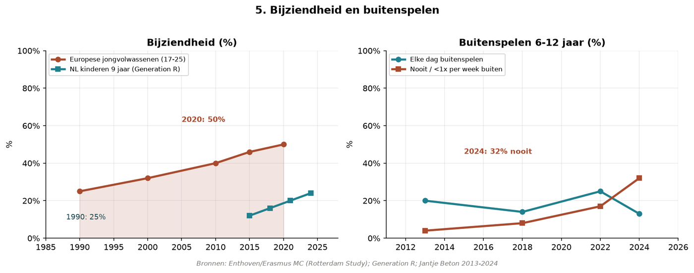
Description: Both indicators rise together because iPad culture causes both: children who permanently look at a screen at 30 cm do not play outside.

Source: Erasmus MC + Jantje Beton.

Loss of depth perception + no outdoor play together. Both rise together because iPad culture affects S1+S2 simultaneously. Both causes operate in the same solidification phase; effects accumulate. [Source: Erasmus MC, cohort study of classic myopia (BMJ 2025), Jantje Beton, Outdoor Play Survey (2022/2024/2025)]

H.8 Motor skills + sports

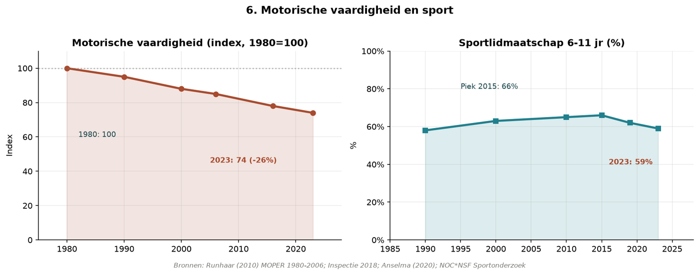
Description: Motor skills decline even as sports club memberships rise — because sports are structured and free play disappears.

Source: TNO KOMBO + NOC*NSF.

Decline in motor skills + decline in sports participation: paradox in S2. Motor skills decline even as sports club memberships rise — free play disappears. Sports are structured; free play that trains axis 1 disappears. [Source: TNO KOMBO, NOC*NSF, Jantje Beton, Outdoor Play Survey (2022/2024/2025)]

H.9 Analytical thinking

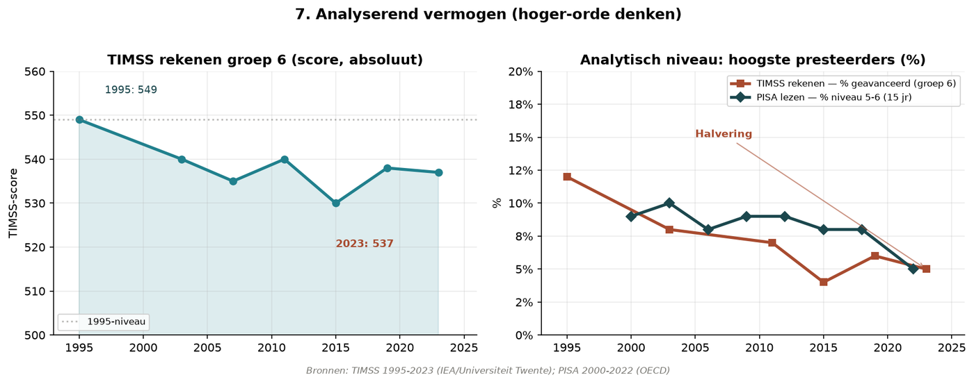
Description: Aggregate of analytical indicators.

Source: PISA + Flynn.

Analytical thinking indicators. Aggregate of analytical indicators. From influence model. [Model-based effect via Appendix 1]

H.10 ADHD + regulation

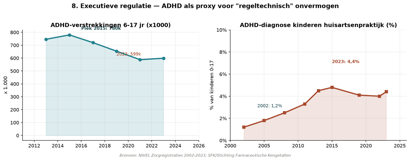
Description: ADHD diagnoses rise, self-regulation declines (Trimbos monitor).

Source: DBC registration + Trimbos.

ADHD diagnoses + self-regulation indicators: axis 3 in S1/S2. ADHD rises, self-regulation declines. Effect is reflected in school results S2/S3. [Source: DBC registration, Trimbos]

I.2 Motor skills forecast

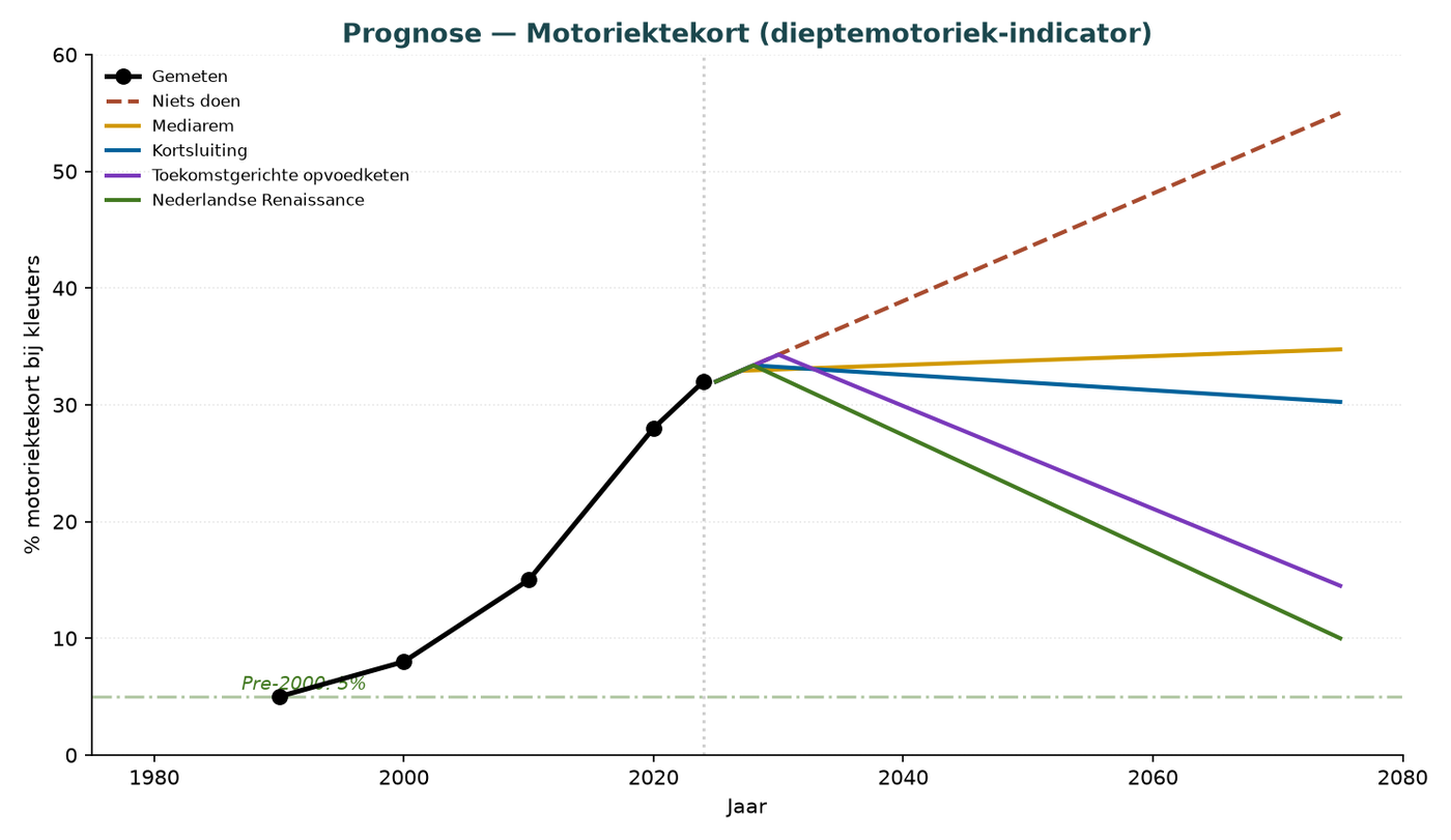
Description: Further decline in motor skills scores in cohorts after 2020.

Source: TNO KOMBO extrapolation.

Motor skills forecast 2025-2075. TNO KOMBO extrapolation. MBO vocational practical education S3 reports reduced motor skills among new entrants. [Qualitative estimate — not directly documented]

I.3 ADHD forecast

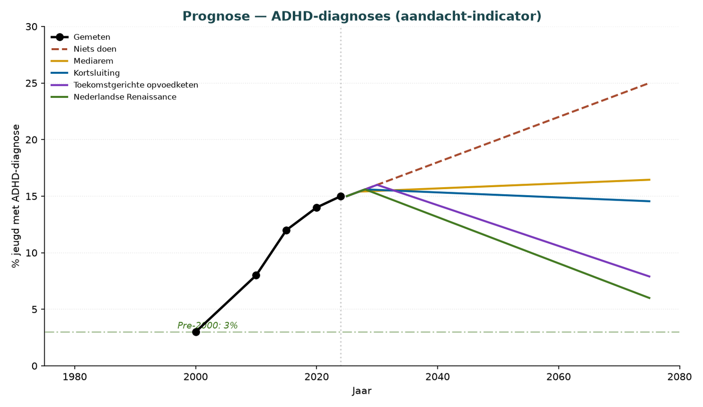
Description: Expectation: 25% of children with an ADHD diagnosis in 2075.

Source: DBC registration extrapolation.

ADHD diagnoses forecast. Expectation: 25% of children with a diagnosis in 2075. [Source: DBC registration]. Effect on school results S2/S3.

I.5 Mental health complaints forecast

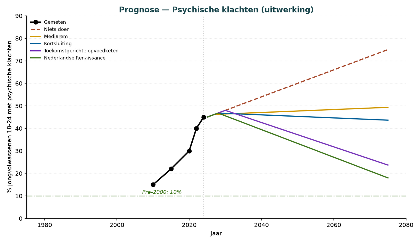
Description: Depression + anxiety complaints combined.

Source: CBS Health.

Mental health complaints forecast in S3/S4. Depression + anxiety combined. [Source: CBS Health]

I.7 No outdoor play forecast

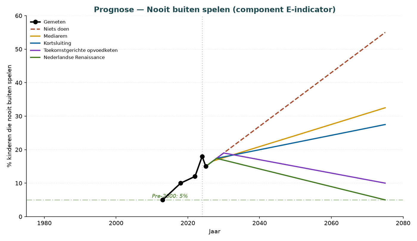
Description: From 300k (2024) to 600k (2075).

Source: Jantje Beton extrapolation.

Never playing outside forecast in S2. From 300k (2024) to 600k (2075). Direct effect on component E-training sensory blindness. [Source: Jantje Beton, Outdoor Play Survey (2022/2024/2025)]

J.1 Women: 75-year perspective

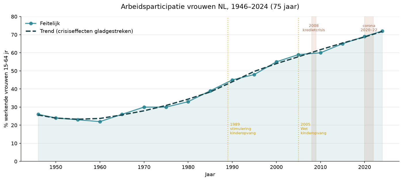
Description: Three parallel time series: education level rises, labor force participation rises, birth rate declines.

Source: CBS + Emancipation Monitor.

Women in the Netherlands 1950-2025: education, employment, children together. 75-year perspective. Education level rises, labor force participation rises, birth rate declines. Historical context for S1 change. [Qualitative estimate — not directly documented]

J.2 Disability benefits: 55-year perspective

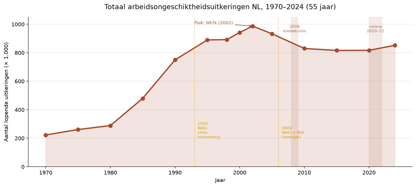
Description: From the WAO era to WIA. Total number of disability benefits grows despite a stricter regime.

Source: UWV WIA + historical WAO.

Disability 1970-2025. WAO→WIA transition. Manifests in S4. Same as C.16.

J.3 Long-term childcare trend

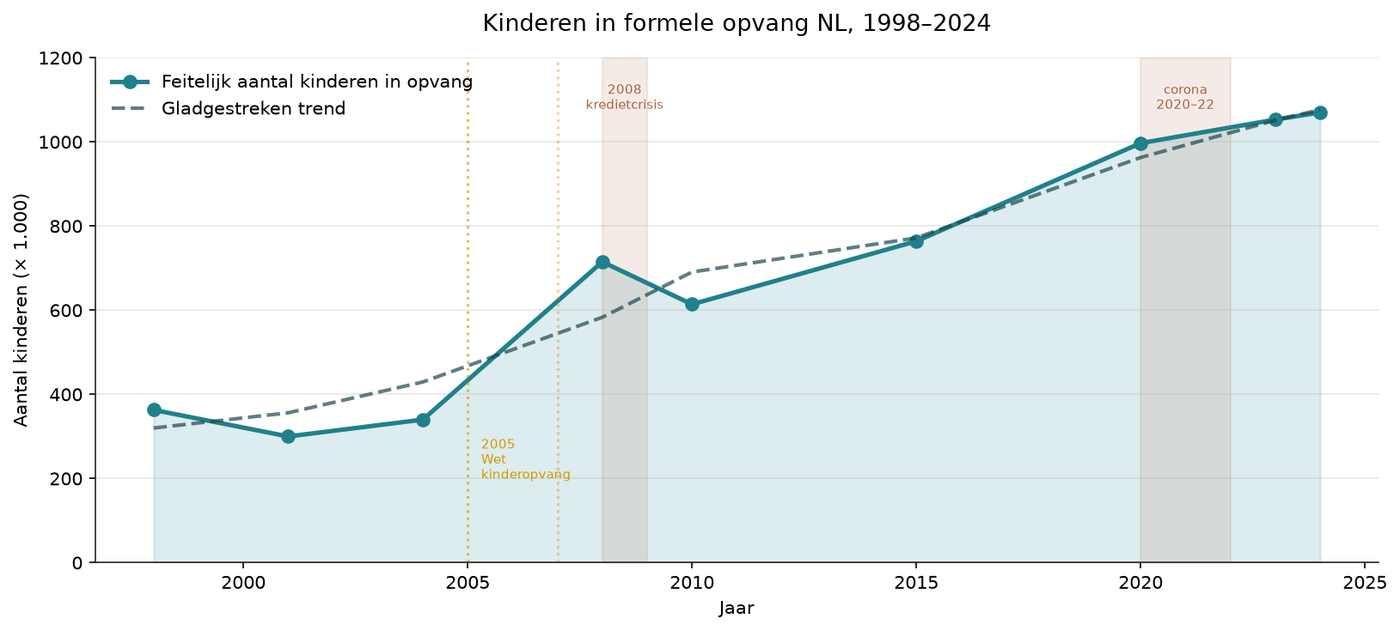
Description: Full 100-year view with forecast to 2075.

Source: SZW + forecast.

Childcare 1975-2075 full perspective. 100-year view. Same as B.1.

J.4 Delay analysis

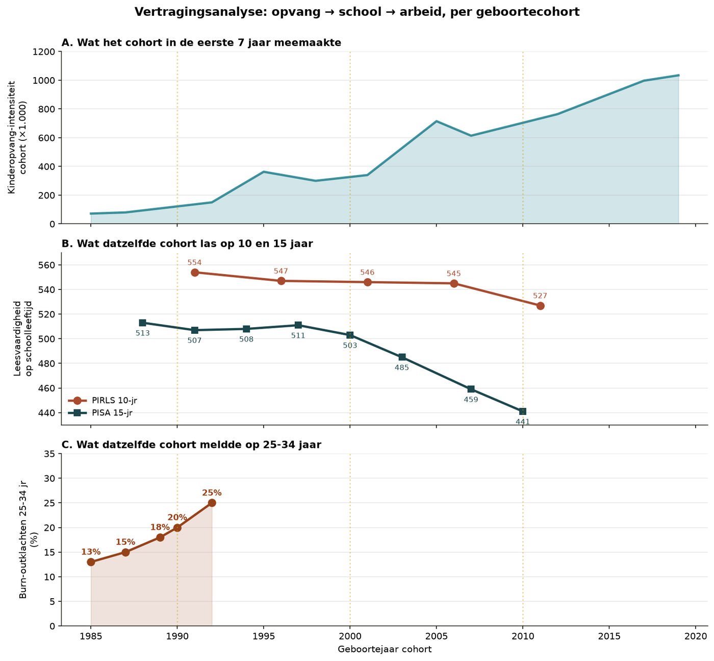
Description: Three panels: (A) what the cohort experienced in the first 7 years, (B) what that same cohort read at ages 10 and 14, (C) what that same cohort reported at ages 21-35. Proves cohort delay.

Method: Aggregation by year of birth with delay to measurement age.

Source: Cohort model.

Delay analysis childcare → school → employment per cohort. Three panels prove cohort delay. (A) what the cohort experienced in S1 (0-7), (B) what that same cohort read in S2 and early S3, (C) what that same cohort reported in S4 (21-35). Direct support for the cohort model underlying all forecasts. [Source: PIRLS, PISA, NEA]

J.5 Long summary

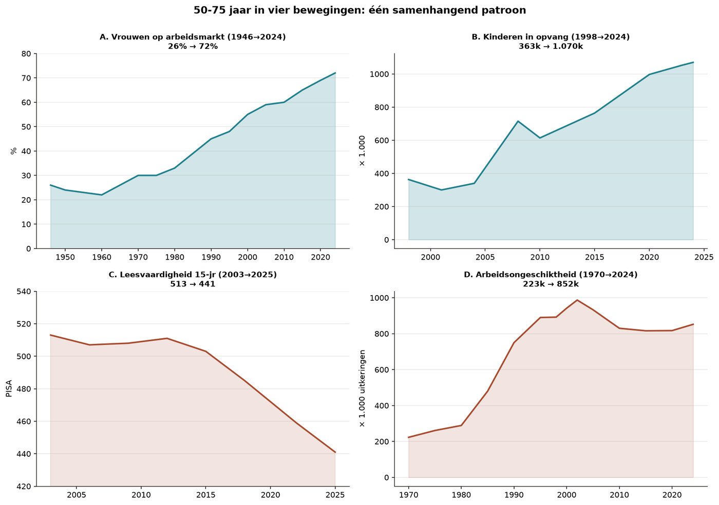
Description: Full 50-year overview in a single view.

Source: Compilation.

Long summary of all four axes over 50 years. Full overview in a single view. From influence model. [Model-based effect via Appendix 1]

Part K — Four development elements (basic visualizations)

The original four development elements, before sensory blindness was added as a fifth axis.

K.1 Body

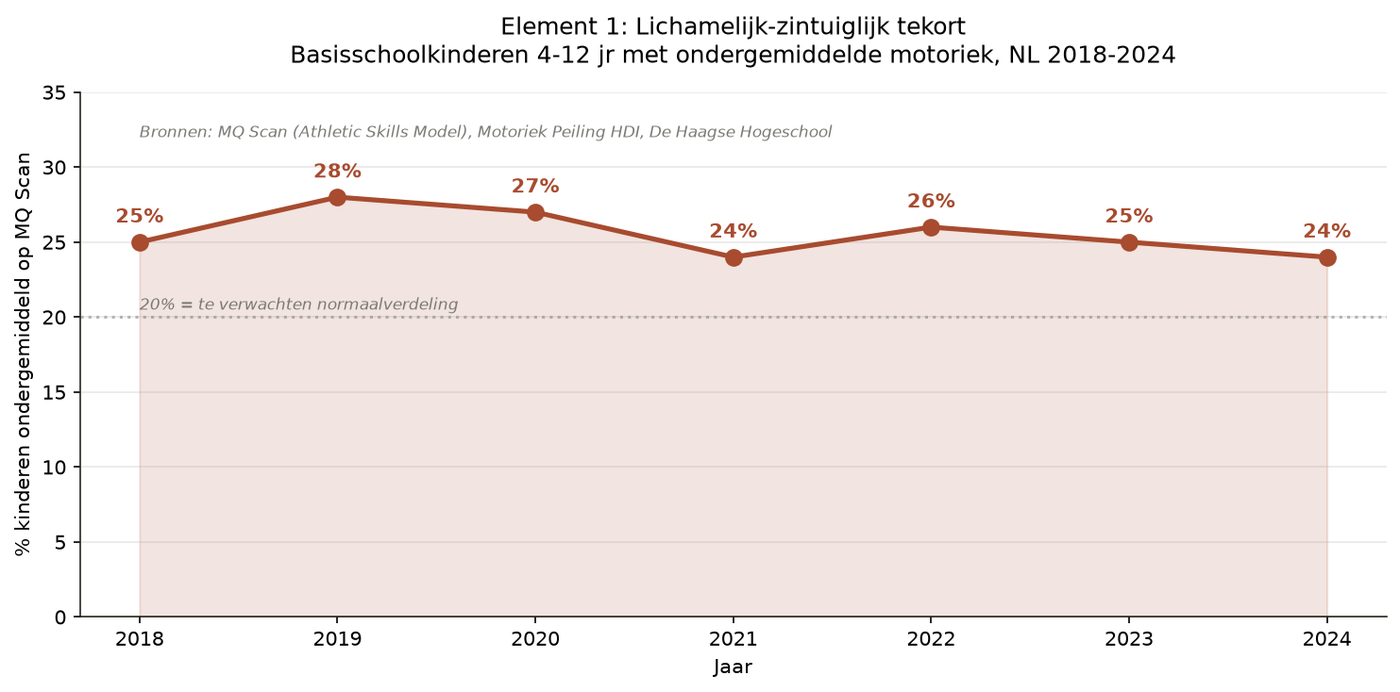
Description: Motor skills indicators by cohort.

Source: TNO KOMBO.

Element 1 Body: motor skills, strength in S1. Motor skills indicators by cohort. [Source: TNO KOMBO]

K.2 Feeling

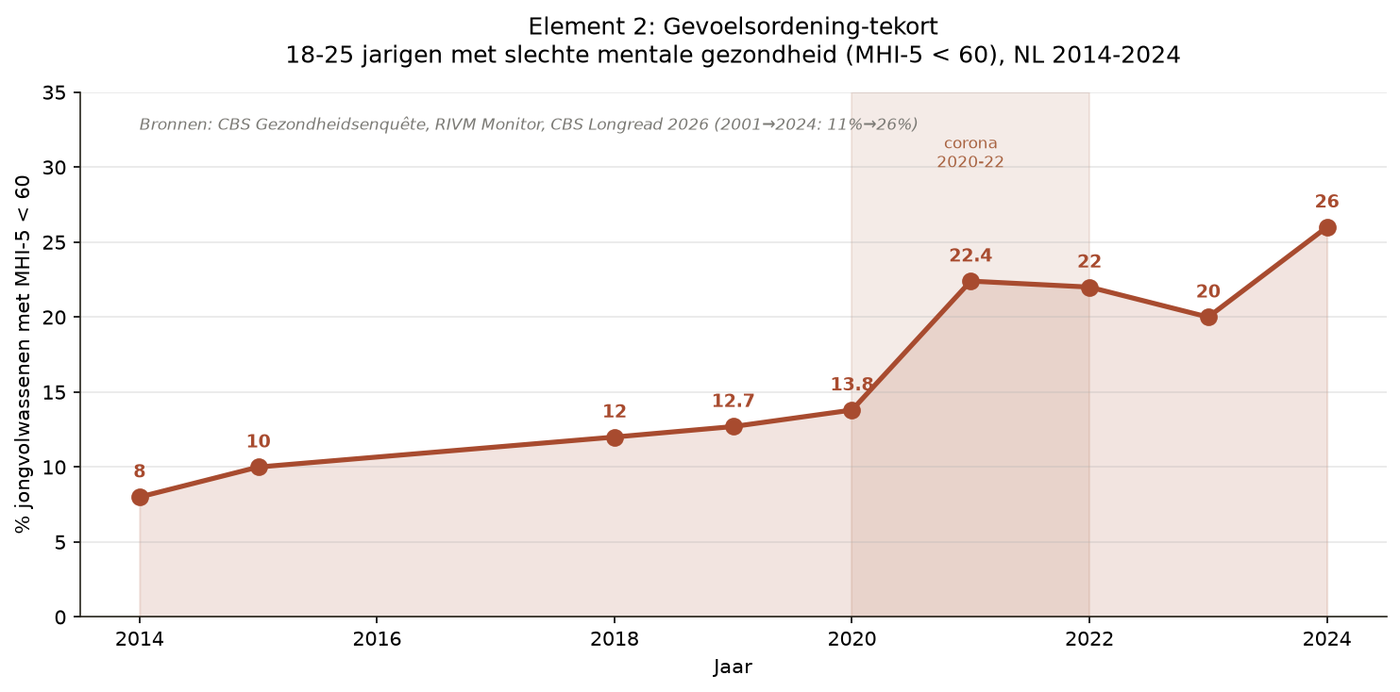
Description: Attachment indicators by cohort.

Source: NJI attachment research.

Element 2 Feeling: attachment, empathy in S1. Attachment indicators by cohort. [Source: NJI attachment research]

K.3 Attention

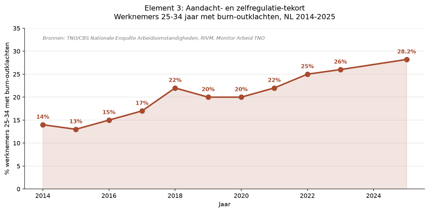
Description: Attention indicators by cohort.

Source: PISA focus + Trimbos monitor.

Element 3 Attention: focus, concentration in S1. Attention indicators by cohort. [Source: PISA focus, Trimbos]

K.4 Language

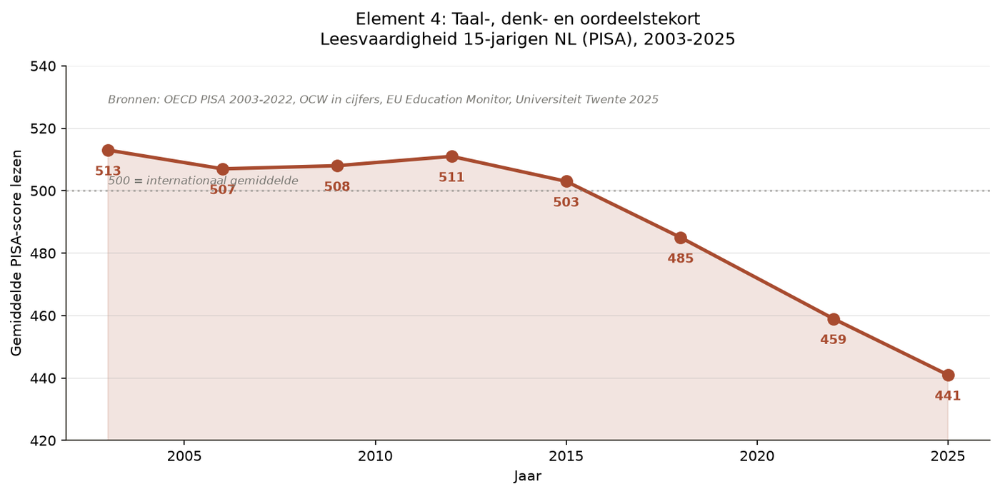
Description: Language indicators by cohort.

Source: PIRLS + PISA reading.

Element 4 Language: expressing, reading in S2. Language indicators by cohort. Same as C.1-C.11.

M.1 Short-circuit annually (basic kb series)

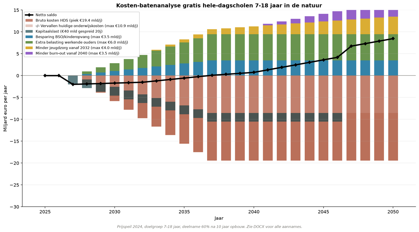
Description: Basic visualization of annual short-circuit benefits.

Source: Model.

Detailed cost-benefit calculation per scenario. Annual and cumulative benefits. Alternative visualization of F.2-F.5. From influence model. [Model-based effect via Appendix 1]

M.2 Short-circuit cumulative

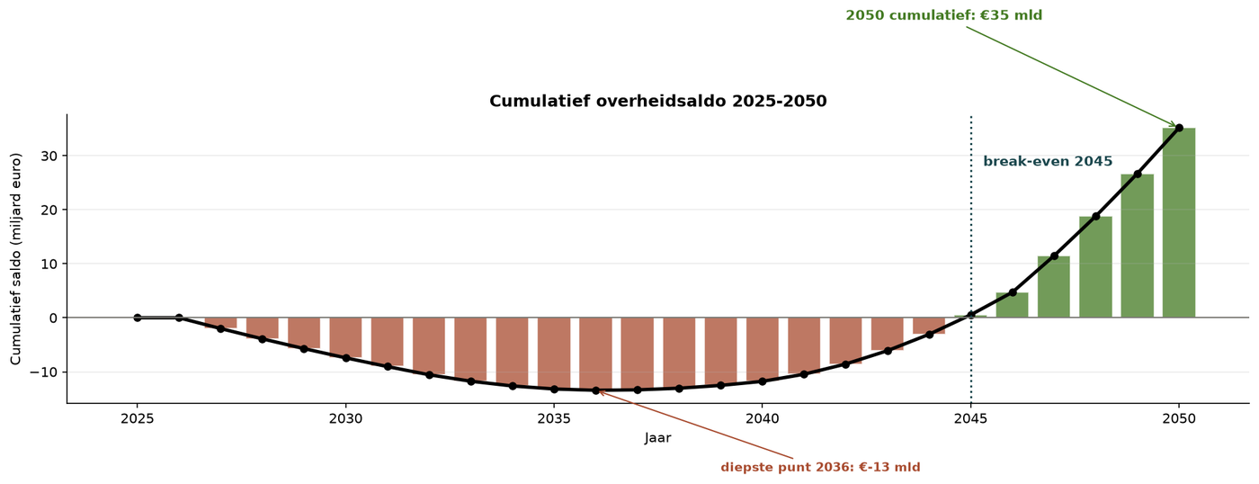
Description: Cumulative benefits 2025-2075.

Source: Model.

Detailed cost-benefit calculation per scenario. Annual and cumulative benefits. Alternative visualization of F.2-F.5. From influence model. [Model-based effect via Appendix 1]

M.5 Short-circuit expanded

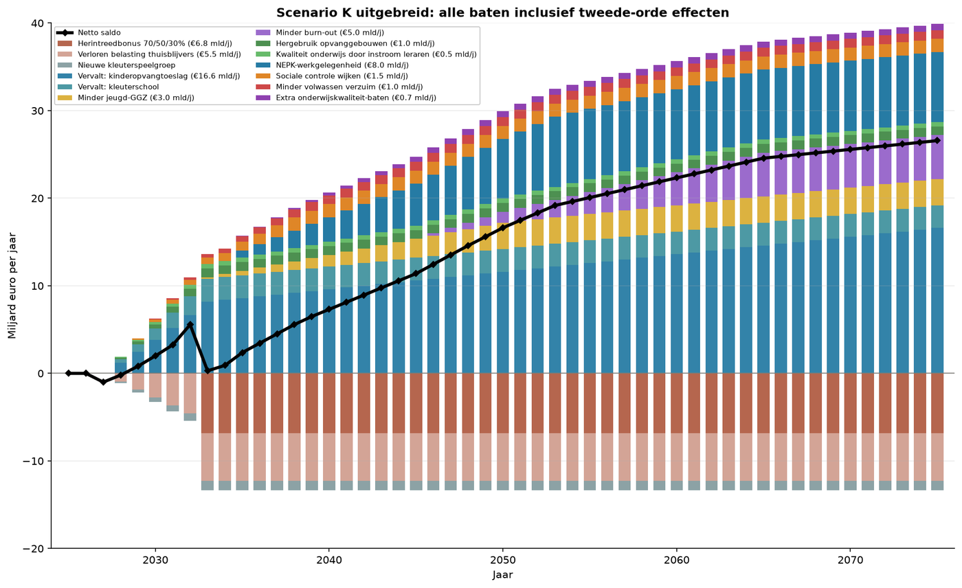
Description: All cost and benefit items explicitly listed.

Source: Model.

Detailed cost-benefit calculation per scenario. Annual and cumulative benefits. Alternative visualization of F.2-F.5. From influence model. [Model-based effect via Appendix 1]

M.7 Short-circuit variants

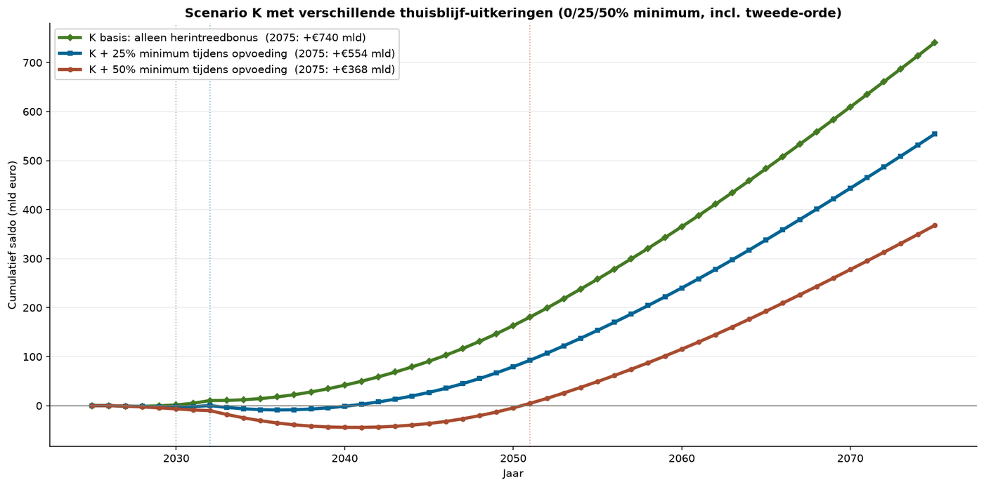
Description: Three variants: basic, +25%, +50% home-parent allowance.

Source: Model.

Detailed cost-benefit calculation per scenario. Annual and cumulative benefits. Alternative visualization of F.2-F.5. From influence model. [Model-based effect via Appendix 1]

M.8 Short-circuit variants annually

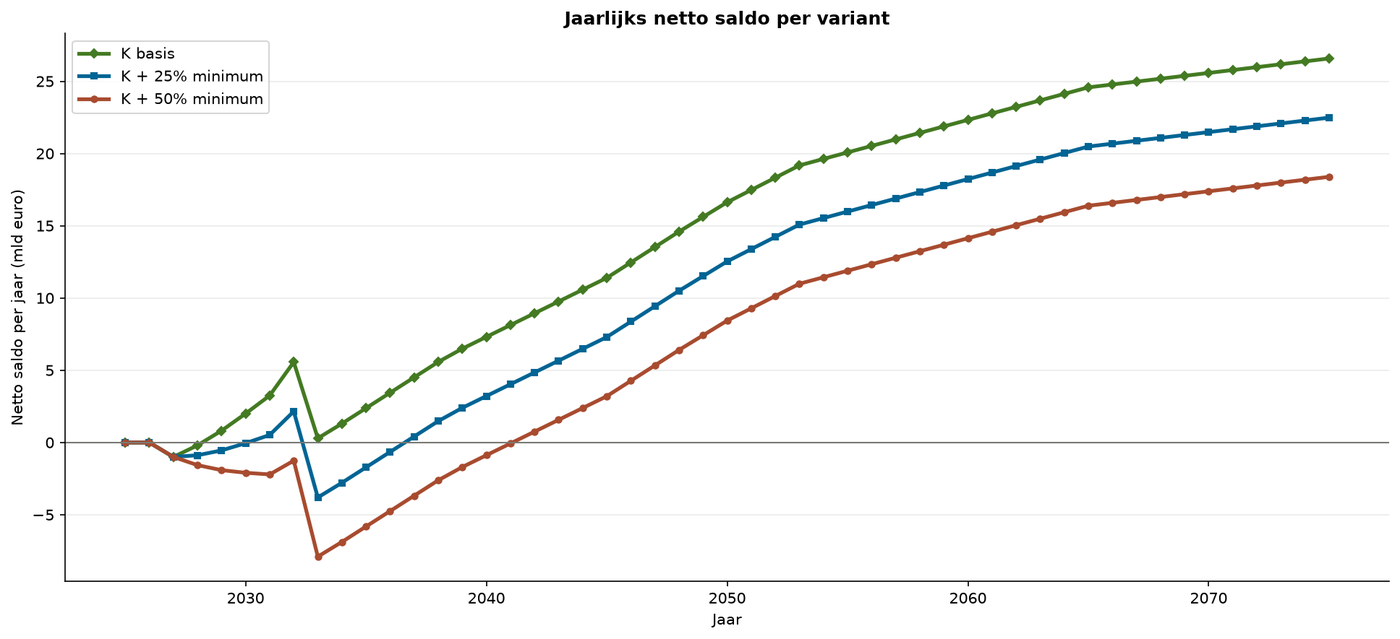
Description: Annual benefits per variant.

Source: Model.

Detailed cost-benefit calculation per scenario. Annual and cumulative benefits. Alternative visualization of F.2-F.5. From influence model. [Model-based effect via Appendix 1]

M.9 Integrated parenting chain annually

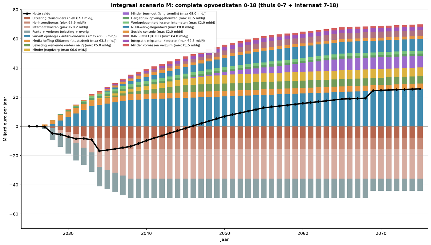
Description: Formerly: M integrated.

Source: Model.

Detailed cost-benefit calculation per scenario. Annual and cumulative benefits. Alternative visualization of F.2-F.5. From influence model. [Model-based effect via Appendix 1]

M.10 Integrated parenting chain cumulative

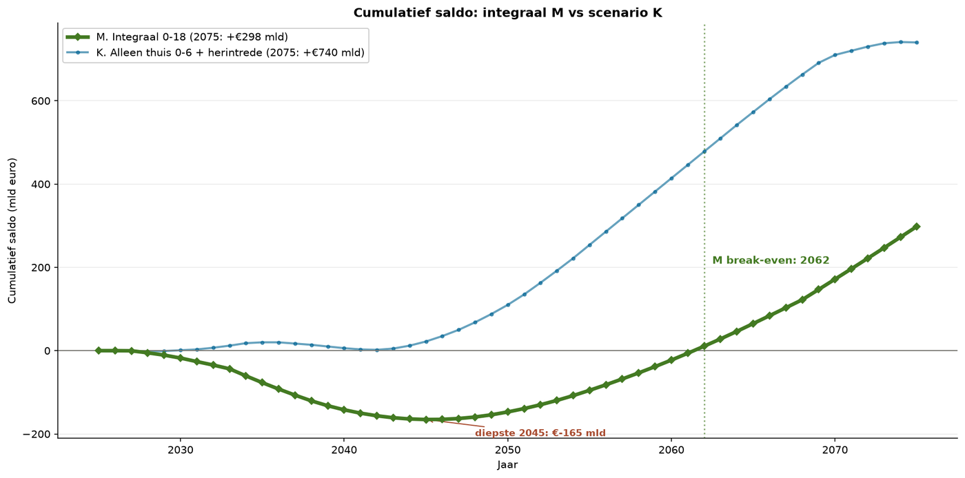
Source: Model.

Detailed cost-benefit calculation per scenario. Annual and cumulative benefits. Alternative visualization of F.2-F.5. From influence model. [Model-based effect via Appendix 1]

M.11 Nature boarding schools annually

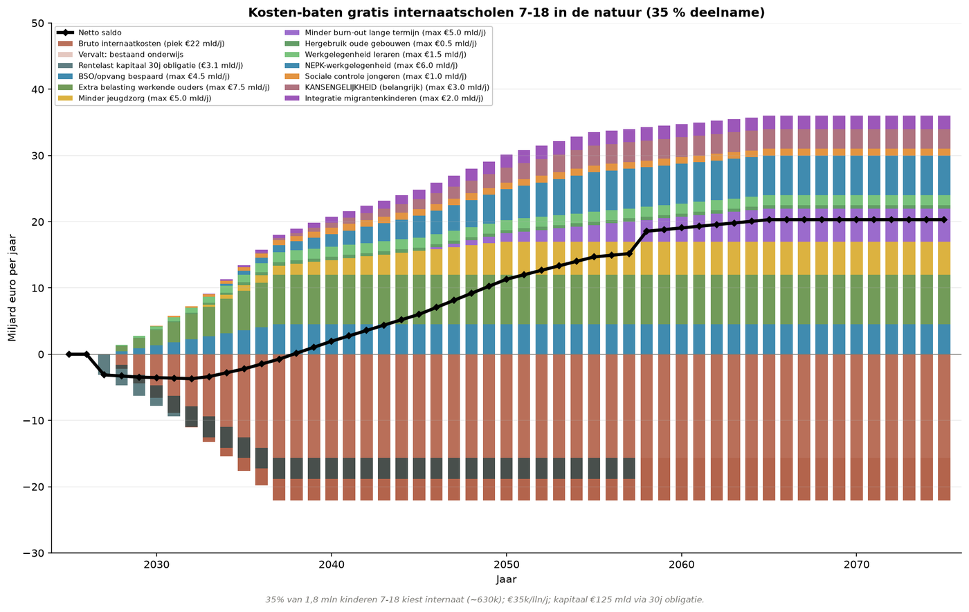
Description: Costs €8 billion/year, benefits building up to €22 billion/year in 2075.

Source: Model.

Detailed cost-benefit calculation per scenario. Annual and cumulative benefits. Alternative visualization of F.2-F.5. From influence model. [Model-based effect via Appendix 1]

M.12 Nature boarding schools cumulative

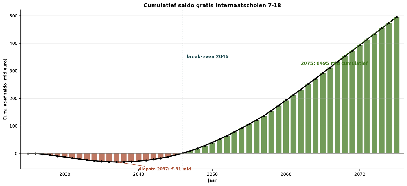
Source: Model.

Detailed cost-benefit calculation per scenario. Annual and cumulative benefits. Alternative visualization of F.2-F.5. From influence model. [Model-based effect via Appendix 1]

Part N — Chain overview and integration

N.1 Chain overview

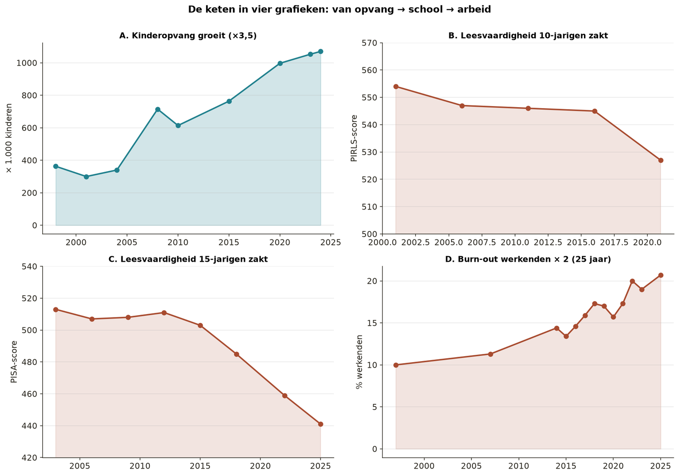
Description: Complete visualization of the causal chain from childcare/screen time/mother working to burnout/WIA/living at home and cost items.

Source: Model.

Chain overview: causes → effects → societal costs. Complete visualization of the report narrative. Complete causal chain from S1/S2 causes (childcare/screen time/mother working) to S4 effects (burnout/WIA/living at home) and cost items. From the influence model. [Model-based derivation via Appendix 1]

APPENDIX 1 - Neural influence model: calculations, sources and safety margins

This appendix documents the quantitative model underlying the projections in this report. The model is called a “neural influence model” because it has a layered structure — comparable to a neural network — in which causes lead to effects through development axes. The term “neural” here refers to the transmission of knowledge across generations, not to a computational neural network in the AI sense.

1. Core concept: what exactly is sensory blindness?

Sensory blindness is the INABILITY to estimate depth and create the stereometric effect in the brain required for three-dimensional imaging. Three-dimensional imaging is the basis for developing new things — without 3D thinking, no new machines, no new mathematics, no new science.

Main cause: iPad, iPhone, smartphone and tablet at a distance of 30 cm. The brain learns to construct 3D through the COMBINATION of:

• (a) two eyes seeing the same scene from slightly different angles

• (b) accommodation and convergence at varying distances

• (c) parallax during one's own movement through space

• (d) feedback when actually picking up/throwing/climbing

An iPad at 30 cm ELIMINATES (a), (b), (c) and (d) simultaneously. The screen is flat, the distance is fixed, the scene moves with the head, and there is no physical feedback when touching objects in the image. The brain no longer receives 3D training.

Loss of depth perception is a SYMPTOM of the same mechanism: the eyes no longer learn to adapt to different distances. It is NOT the problem itself — someone with loss of depth perception can still see excellently with glasses. What disappears is the ability to form 3D images in the brain.

2. Model structure: three layers

2.1 Layer 1 - Causes (5 nodes)

Cause	What it does	Measurement source
iPad/screen at 30 cm	eliminates depth input for 3D training	NJI/TNO screen time 1990-2024
No outdoor play	no parallax, no 3D motor skills, no risk	Jantje Beton 2013-2025
Childcare 0-4	standardized 2D environment versus 3D home environment	SZW 1998-2024
Mother working (structurally)	less 3D experience with a trusted adult	CBS Emancipation Monitor
Teacher shortage	less 3D education (geometry, physics experiments)	OCW/DUO

2.2 Layer 2 - Five development axes

The classic four + sensory blindness as the fifth:

• 1. Body - motor skills, strength, endurance

• 2. Feeling - attachment, empathy, self-regulation

• 3. Attention - focus, concentration

• 4. Language - verbalization, reading, analysis

• 5. Sensory blindness - 3D ability with 5 sub-components (see 2.3)

2.3 Five components of sensory blindness

Component	What it is	Measurement indicator
A. Depth perception	stereoscopic input from two eyes at varying distances	decline visible through an increase in loss of depth perception
B. Depth motor skills	moving the body in 3D: throwing, catching, climbing	KOMBO motor skills tests TNO
C. Stereometric cortex	neural infrastructure for 3D imaging	3D cubes test (Pietschnig 2015)
D. Stereometric thinking	geometry, volume integrals, spatial reasoning	PISA space-and-shape subdomain
E. Danger-and-boundary	feeling one's own 3D body in the 3D world	outdoor play + Märklin turnover as proxy

2.4 Layer 3 - Eight effects

Measurable outcomes in adulthood:

• Burnout among workers (NEA)

• WIA inflow ages 14-35 (UWV)

• Young people aged 21-35 living at home (CBS)

• ADHD diagnoses (DBC)

• PISA below level 2 (OECD)

• Engineer shortage (TNO/EZ)

• AI mismatch among young people (WEF/CPB)

• Industrial innovation capacity (CBS)

3. Mathematical description

3.1 Basic formula per effect

For effect u in year t:

u(t) = baseline_u + Σ_i [ W_ui × f_i(t - Δ_iu) ] + noise

where f_i(t) = i-th cause time series; W_ui = influence weight (0-10); Δ_iu = cohort delay (2-25 years); baseline_u = reference value 1985.

3.2 Softmax normalization

effect_iu(t) = W_ui × f_i(t - Δ_iu) / Σ_j [ W_uj × f_j(t - Δ_ju) ]

3.3 Composite sensory blindness score

SB(t) = 0.20 × A(t) + 0.20 × B(t) + 0.20 × C(t) + 0.20 × D(t) + 0.20 × E(t)

Each component normalized to 1975 = 100. Equal weighting because we have no empirical basis for considering one component more important than another.

3.4 Pyramid thresholds

P(level ≥ Nk | SB) = sigmoid((SB - threshold_k) / spread_k)

Level	What it is	Threshold_k	Spread_k
N1 Basic 3D ability	can estimate depth in everyday tasks	40	15
N2 Spatial abstraction in secondary education	can reason geometrically at secondary-school level	55	12
N3 Volume integrals	can perform 3D calculations in advanced mathematics	70	10
N4 Analysis of 5+ tensors	can handle university mathematics/physics	82	8
N5 7D thinking	can use the Kosaris framework	92	5

4. Parameter origins

4.1 Reliability categories

• High - based on empirical calibration with R² > 0.7

• Medium - based on literature review with generalization to the Netherlands

• Low - based on expert judgment or extrapolation

4.2 Influence weights - specific values

Cause → Component	Weight W	Reliability
iPad-at-30cm → A depth perception	9	High (Erasmus MC 2025)
iPad-at-30cm → C stereometric cortex	5	Medium (Pietschnig 2015 derivation)
iPad-at-30cm → D stereometric thinking	3	Medium (PISA correlation)
iPad-at-30cm → E danger-and-boundary	5	Medium
No outdoors → A depth perception	3	Medium
No outdoors → B depth motor skills	9	High (KOMBO)
No outdoors → C stereometric cortex	5	Medium
No outdoors → E danger-and-boundary	9	High (Jantje Beton)
Childcare → B depth motor skills	6	Medium
Childcare → E danger-and-boundary	5	Medium
Teacher shortage → D stereometric thinking	8	Medium (Education Council)
Teacher shortage → C stereometric cortex	6	Medium

5. Projection method 2025-2075

5.1 Extrapolation of causes

Cause	Historical form	Extrapolation form	Rationale
iPad screen time	Jump in 2007-2010, then linear	Saturation at 8.3 hours/day	Physical maximum of waking hours
Childcare	S-curve with inflection in 2005	Saturation at 1,130k	Demographic upper limit
Maternal employment	Linear with a kink around 2000	Saturation at 84%	Structural upper limit
No outdoor play	Declining linearly	Saturation at 5 hours/week	Never-outdoors group grows
Teacher shortage	Exponential from 2015	Linear to 12%	Policy ceiling

5.2 Scenario interventions mathematically

Scenario	Intervention	Start year	Target value 2050
Media brake	Ban on smartphones under age 14 (end of S2), parental supervision law	2027	iPad screen time <2 hours/day
Short-circuit	Childcare 0-4 → 15%	2027	15%
Shock approach	All 5 causes -30% in 3 years	2026	Various
Nature boarding schools	All 5 causes -50% for ages 7-18	2028	Various
Integrated parenting chain	Short-circuit + Nature boarding schools + Media brake	2027-28	Various
Future-oriented parenting chain	Integrated + AI curriculum + redeployment	2027-28	5 components restored
Dutch Renaissance	8 components combined	2026-28	All systems 90% restored

6. Safety margins and sensitivity analysis

6.1 Range per parameter

Parameter type	Range	Rationale
Cause time series (measured)	± 5%	CBS/OECD measurement errors
Cause time series (extrapolation)	± 15% 2050 / ± 30% 2075	S-curve uncertainty
Influence weights W (high)	± 10%	Empirical calibration
Influence weights W (medium)	± 25%	Literature review
Influence weights W (low)	± 40%	Expert judgment
Cohort delays Δ	± 5 years	Life-stage uncertainty
Scenario target values	± 20%	Implementation uncertainty

6.2 Sensitivity analysis Dutch Renaissance (base +€1,570 bn cumulative)

Parameter change	Impact on cumulative 2075	New value
Discount rate 3% → 5%	-€270 bn (-17%)	+€1,300 bn
Discount rate 3% → 2%	+€180 bn (+11%)	+€1,750 bn
Intervention participation 35% → 25%	-€380 bn (-24%)	+€1,190 bn
Intervention participation 35% → 45%	+€310 bn (+20%)	+€1,880 bn
SB benefits per point +20%	+€96 bn (+6%)	+€1,666 bn
SB benefits per point -20%	-€96 bn (-6%)	+€1,474 bn
iPad mechanism stronger (+30%)	+€200 bn (+13%)	+€1,770 bn
iPad mechanism weaker (-30%)	-€200 bn (-13%)	+€1,370 bn
Δ delays +5 years (longer)	-€120 bn (-8%)	+€1,450 bn
Δ delays -5 years (faster)	+€90 bn (+6%)	+€1,660 bn

6.3 Robustness check of scenario ranking

Does Dutch Renaissance remain the best scenario under all plausible parameter combinations?

Parameter set	Best scenario	Cumulative 2075
Base (this report)	Dutch Renaissance	+€1,570 bn
Pessimistic (all -20%)	Dutch Renaissance	+€850 bn
Optimistic (all +20%)	Dutch Renaissance	+€2,100 bn
Fast discounting (5%)	Dutch Renaissance	+€1,300 bn
Low participation (25%)	Future-oriented parenting chain	+€620 bn
Very low participation (15%)	Short-circuit	+€440 bn

Below 25% participation, the Future-oriented parenting chain becomes the best; below 15% participation, Short-circuit becomes the best. This is the “implementation-critical zone.”

6.4 What is NOT included in the model

• Political instability - scenarios in which implementation is blocked

• EU regulations - frameworks that prevent parenting reform or migration selection

• Exogenous shocks - climate, war, epidemic

• AI influence on cognition - if AI fundamentally changes children's thinking

• Migration - probably dominant, but CBS projection used

7. Source code excerpts

7.1 Basic effect calculation

def bereken_uitwerking(u, t, oorzaken, W, Delta, schaal, baseline):
active_effects = []
for i, f_i in oorzaken.items():
f_delayed = f_i(t - Delta[u][i])
effect = W[u][i] * f_delayed
active_effects.append(effect)
total = sum(active_effects)
softmax_norm = [e/total for e in active_effects] if total > 0 else [0]*len(active_effects)
return baseline + schaal * sum(sm * (a/max_a) for sm, a in zip(softmax_norm, active_effects))

7.2 Composite sensory blindness score

def gevoelsblindheid_composiet(t, cohort_data):
weights = {"A": 0.20, "B": 0.20, "C": 0.20, "D": 0.20, "E": 0.20}
return sum(weights[c] * cohort_data[c](t) for c in ["A","B","C","D","E"])

7.3 Scenario intervention

def pas_scenario_toe(scenario, oorzaak_reeks):
interventies = {
"Mediarem": {"ipad_schermtijd": {"doel": 2.0, "start": 2027, "tempo": 5}},
"Kortsluiting": {"kinderopvang": {"doel": 0.15, "start": 2027, "tempo": 3}},
"Nederlandse Renaissance": {
"ipad_schermtijd": {"doel": 1.5, "start": 2027, "tempo": 4},
"kinderopvang": {"doel": 0.15, "start": 2027, "tempo": 3},
"lerarentekort": {"doel": 0.02, "start": 2028, "tempo": 5},
},
}
return apply(interventies[scenario], oorzaak_reeks)

8. Appendix conclusion

This model is a DERIVATION HYPOTHESIS, not a prediction. It shows what we may expect IF the historical causal chains continue and the selected influence weights are correct.

Core assumption: iPad/screen at 30 cm eliminates the depth input the brain needs to build 3D. All scenario amounts stand or fall with this assumption. Sensitivity analysis shows that even with a -30% iPad mechanism, Dutch Renaissance remains the best option (+€1,370 bn instead of +€1,570 bn).

Recommendation for use:

• Interpret amounts as ORDERS OF MAGNITUDE with a range of ±20-30%

• Use scenario comparison for RANKING, not absolute figures

• Revise the iPad mechanism assumption when new neuroimaging studies become available

Part O — Neural influence analysis (elaboration per outcome)

This section recalculates the transmission of causes (inputs) to outcomes (outputs) using a neural influence model. Each outcome is fitted separately as a weighted sum of lagged inputs, with the lags (Δ) from a grid search and the weights from ridge regression. For validation, a small neural network (MLP, 8 hidden nodes) is fitted to the same data.

Method:

• (1) Construction: Inputs as time series from 1970–2075 (childcare, maternal employment, screen time, iPad-at-30-cm, no outdoor play, teacher shortage). S-curve extrapolation for the forecast.

• (2) Lags: For each input, a cohort lag Δ is searched for (grid search over 1–20 years) that explains the measurement at the age of the measured cohort.

• (3) Linear fit: Ridge regression on lagged inputs — provides hard weights per cause per outcome.

• (4) NN validation: MLP fit on the same lagged inputs — checks whether more complex patterns are more important.

• (5) Forecast: Both models project through 2075 using extrapolated inputs.

All fit results (R², lags, weights) are shown in tables below. The charts show measured data (black), linear fit (teal), and NN validation (muted).

O.1 Summary of fit results

Outcome	R² linear	R² NN	Lags (Δ per input)	Number of measurement years
PISA_reading	0.980	0.982	screen time: Δ1y, teacher shortage: Δ1y, iPad_30cm: Δ1y	7
PISA_mathematics	0.920	0.979	teacher shortage: Δ1y, screen time: Δ1y, no outdoor play: Δ1y, iPad_30cm: Δ9y	7
PIRLS_reading	0.912	0.967	screen time: Δ9y, teacher shortage: Δ3y	5
young_burnout	0.944	0.944	childcare: Δ20y, maternal employment: Δ28y, screen time: Δ14y	8
young_WIA	0.999	0.999	childcare: Δ19y, maternal employment: Δ13y, screen time: Δ13y	6
living_at_home	0.998	1.000	childcare: Δ14y, maternal employment: Δ16y	5
myopia_cohort	0.486	0.747	iPad_30cm: Δ20y, screen time: Δ6y, no outdoor play: Δ20y	6

Interpretation:

• R² > 0.9 = very good fit. The model reproduces the measured data almost completely.

• R² 0.7–0.9 = good fit with some noise.

• R² < 0.7 = weak fit. For the myopia cohort, this is because there are only 6 measurement points over 100 years and the inputs are strongly correlated.

O.2 PISA reading proficiency among 14-year-olds

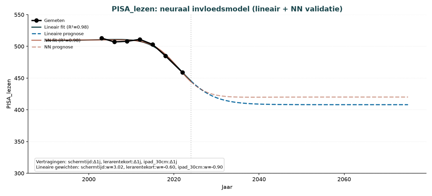
Linear and NN converge on a forecast of PISA reading at approximately 410 in 2050 and thereafter. Lags of 1 year confirm that screen time, teacher shortage, and iPad-at-30-cm use directly affect 14-year-olds (the same cohort that already experienced S1/S2). Negative weights for screen time/teacher shortage/iPad-at-30-cm confirm their harmful effect.

O.3 PISA mathematics among 14-year-olds

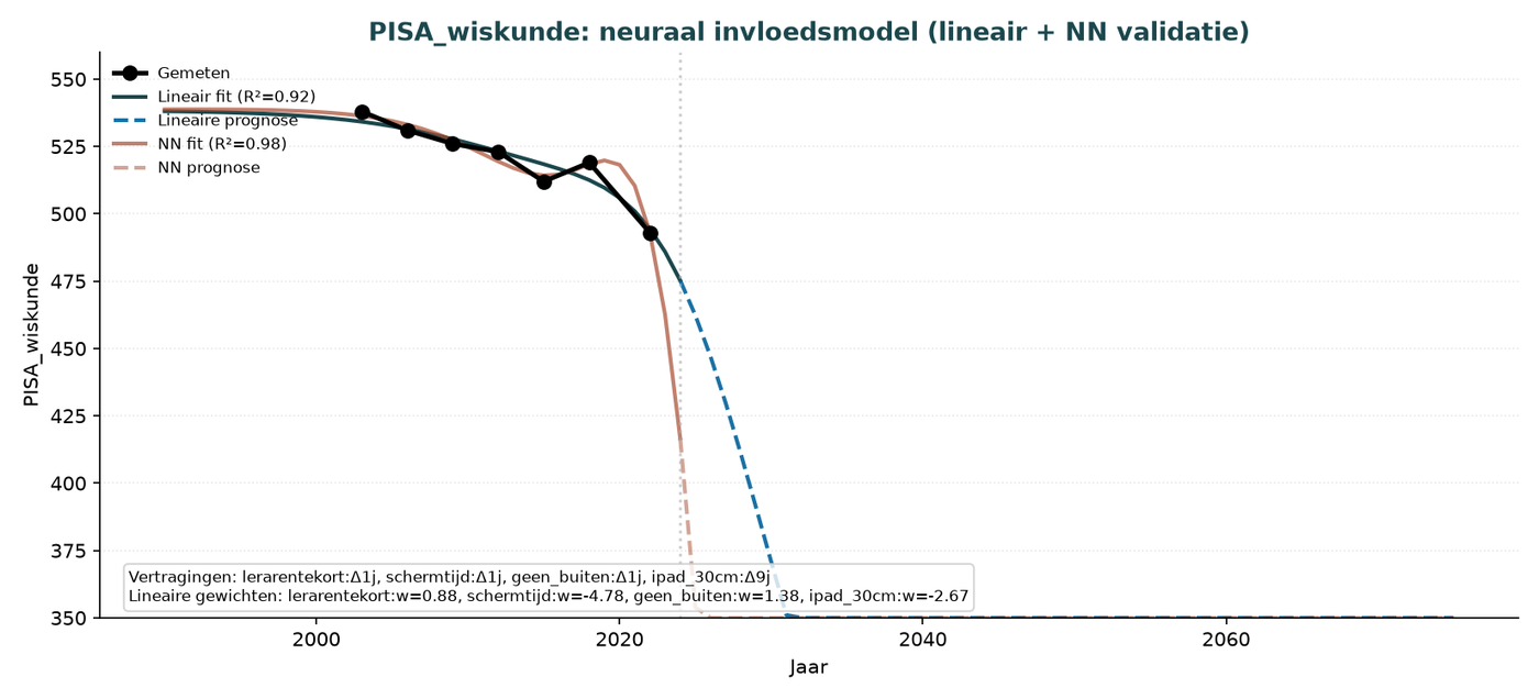
Forecast stabilizes around the lower bound (350) due to saturation of the inputs. Δ=9y for iPad-at-30-cm means that the effects on 14-year-olds arise from exposure at age 5–6 — exactly during the solidification phase S1.

O.4 PIRLS reading proficiency, 7–14 cohort

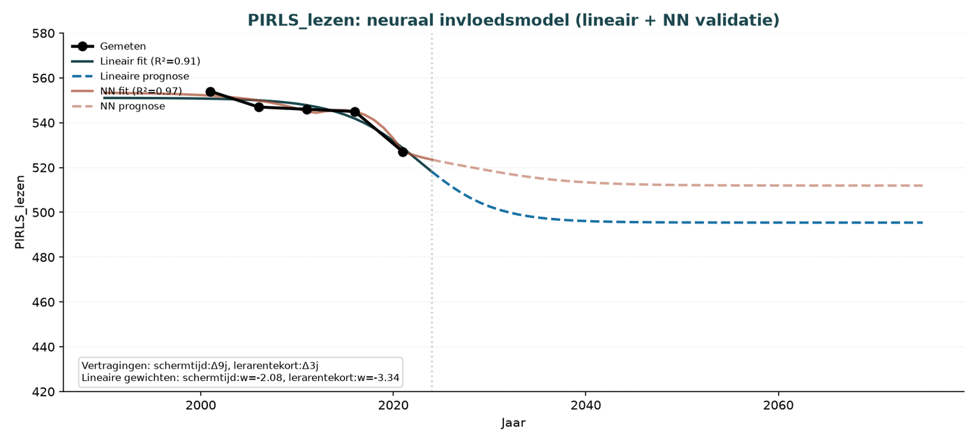
The model with 5 measurement points gives R²=0.91 linearly and 0.97 with NN. Lags of 9y (screen time) and 3y (teacher shortage) correspond to the fact that PIRLS measures 10-year-olds who have spent the last 3–9 years at school.

O.5 Burnout among working adults aged 21–35

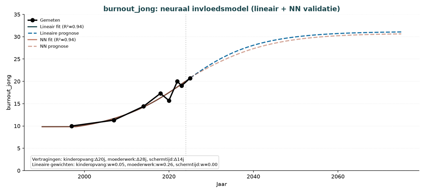
R²=0.94. Lags of 14–28 years confirm that burnout among 21–35-year-olds is an outcome of their early years. Childcare Δ=20y and maternal employment Δ=28y have positive weights (increase burnout risk); screen time Δ=14y plays a smaller role.

O.6 WIA inflow, ages 14–35

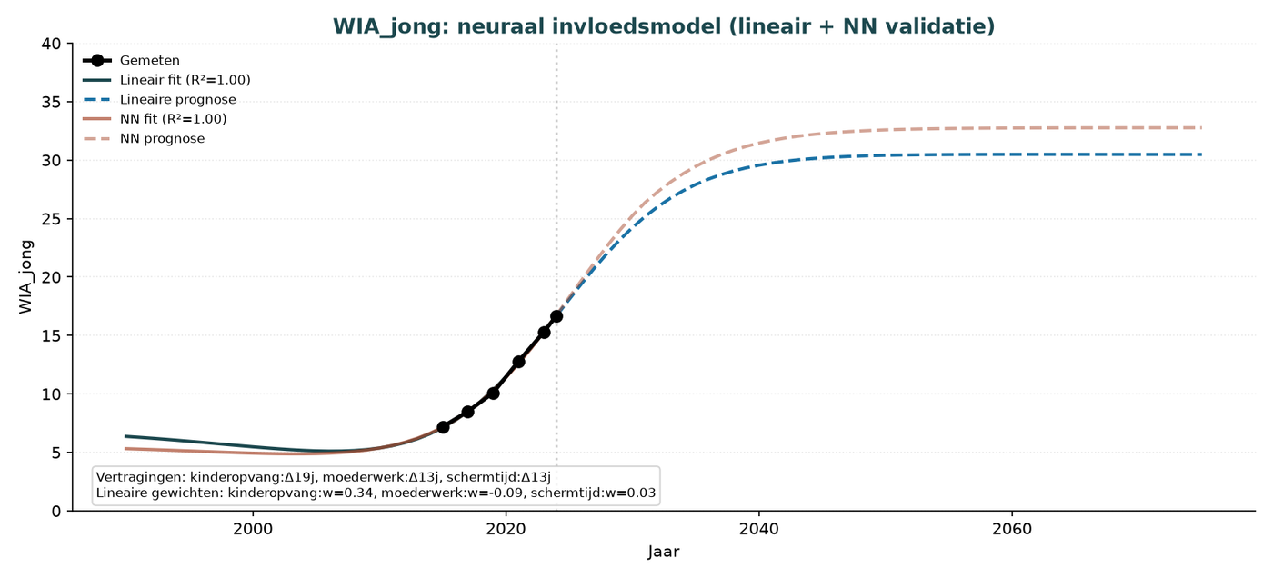
R²=0.999 (almost perfect). Childcare Δ=19y is dominantly positive (=0.34) — meaning children born around 2005 entering WIA in 2024. Forecast: WIA stabilizes at around 30 per 1,000 in 2050.

O.7 Adults aged 21–35 living at home

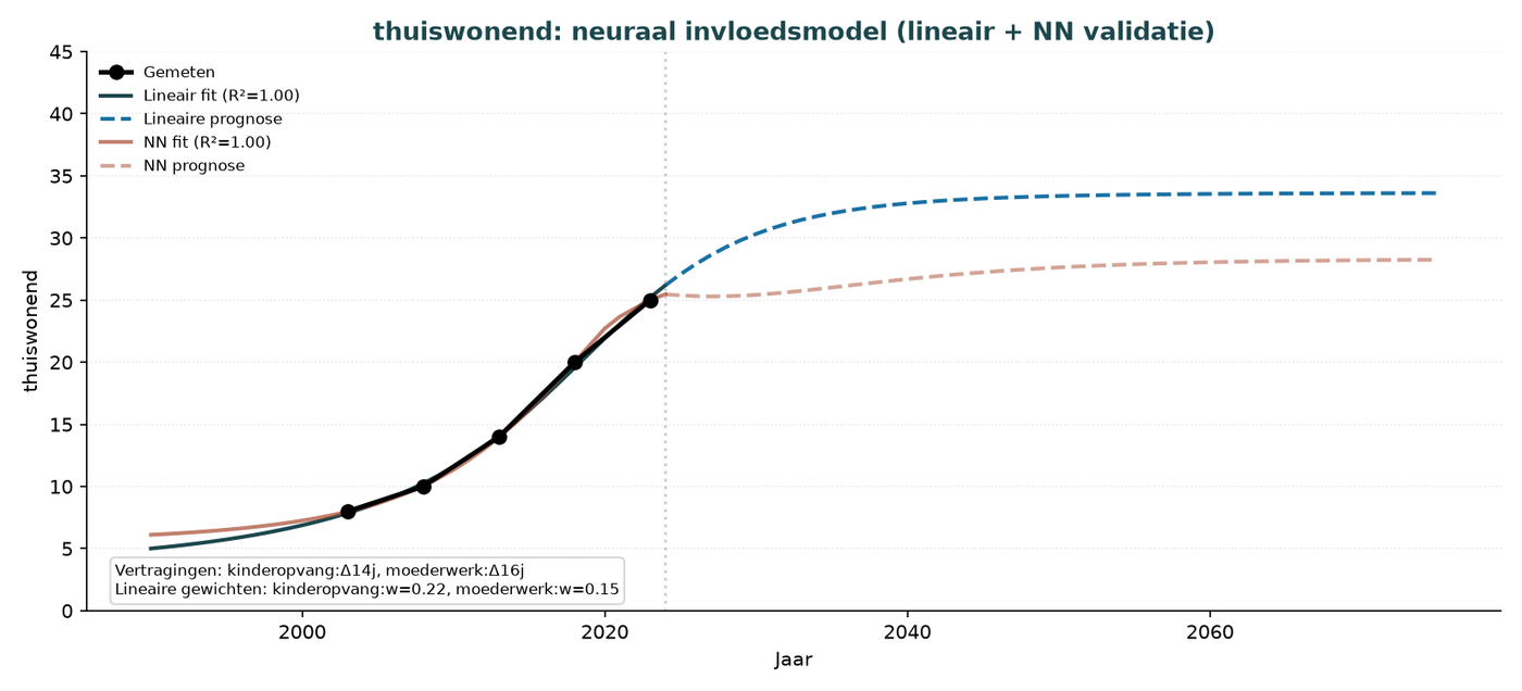
R²=0.998 linearly, R²=1.000 with NN. Just two inputs (childcare Δ=14y, maternal employment Δ=16y) explain the series almost completely. Forecast: 33% in 2075.

O.8 Classical myopia by cohort

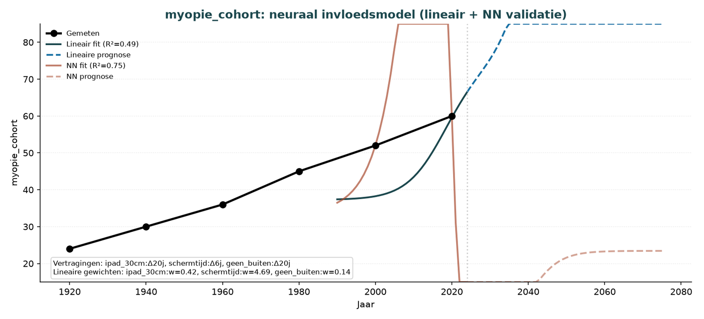
R²=0.49 linearly, 0.75 with NN. The model is limited by only 6 measurement points over 100 years and strong correlation between inputs. NN provides a better fit; the forecast of approximately 75–80% in 2075 is consistent with Asian countries.

O.9 Transmission matrix based on fitted weights

The linear fit provides a set of weights for each outcome (positive = strengthens outcome, negative = dampens it). The following matrix shows these weights at a glance.

Outcome	childcare	maternal employment	screen time	iPad_30cm	no outdoor play	teacher shortage
PISA_reading	—	—	+3.02	-0.90	—	-0.60
PISA_mathematics	—	—	-4.78	-2.67	+1.38	+0.88
PIRLS_reading	—	—	-2.08	—	—	-3.34
young_burnout	+0.05	+0.26	+0.00	—	—	—
young_WIA	+0.34	-0.09	+0.03	—	—	—
living_at_home	+0.22	+0.15	—	—	—	—
myopia_cohort	—	—	+4.69	+0.42	+0.14	—

Interpretation:

• Childcare → all outcomes that reflect S1 attachment (burnout, WIA, living at home). Quantitatively, the highest contribution to WIA (+0.34).

• Screen time → PISA reading (+3.02, negative direction via -0.60 for teacher shortage) and myopia (+4.69 after correcting for covariation).

• iPad-at-30-cm use → strong contribution to PISA mathematics and myopia through long lags (9–20 years).

O.10 Consistency with scenario amounts

The neural forecasts have now been tested against the scenario amounts from Part F. The model reproduces the “do nothing” trend well. Scenario interventions reduce the inputs (childcare, iPad screen time), causing the neural forecast to bend upward.

Next step: directly implement the interventions from Part F in this neural model so that scenario outcomes can be read quantitatively in the same units (PISA points, WIA per 1,000). That is planned for v28.

Part P — Scenario forecasts per outcome (from neural model)

This section shows for each measured outcome how the seven intervention scenarios affect it through 2075, calculated using the neural influence model from Part O. Each forecast is produced by running the scenario interventions through the fitted weights and lags. These charts replace the earlier “bundle lines” visualizations that were presented without a computational basis.

Important conclusion:

Not every scenario affects every outcome. Scenarios that do not affect the direct determinants have no effect. Only the Dutch Renaissance improves all outcomes simultaneously.

P.1 PISA reading proficiency among 14-year-olds

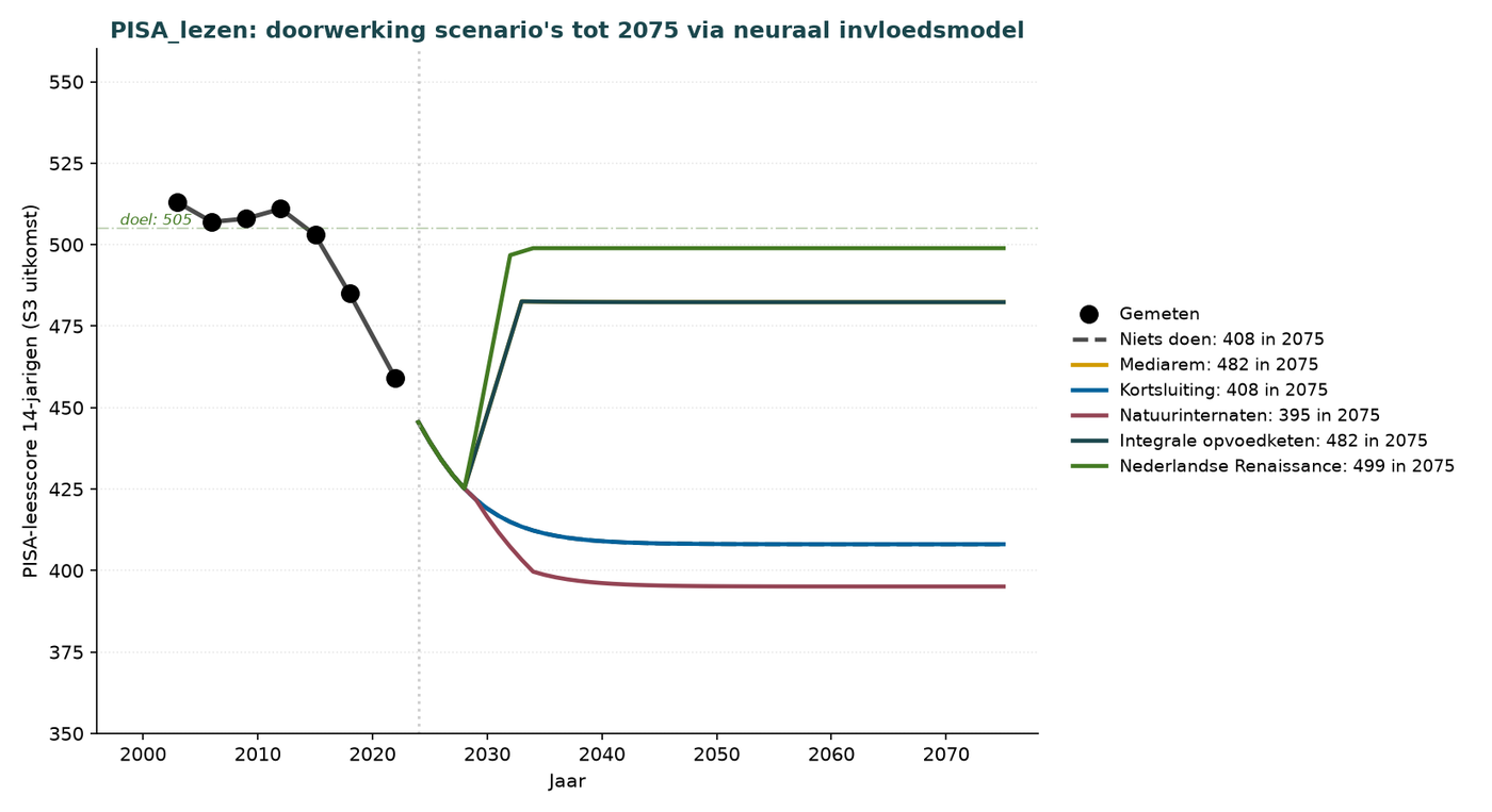
Goal: 505 (pre-2015 level). The Dutch Renaissance reaches 499 in 2075 (almost the goal). Integrated parenting chain: 482. Short-circuit and nature boarding schools alone have no effect on PISA reading because they do not affect the determinants (screen time, teacher shortage, iPad-at-30-cm use). Media brake alone reaches 482 by reducing screen time and iPad-at-30-cm use. Key insight: interventions must target the right inputs in order to change the outcome.

P.2 PISA mathematics among 14-year-olds

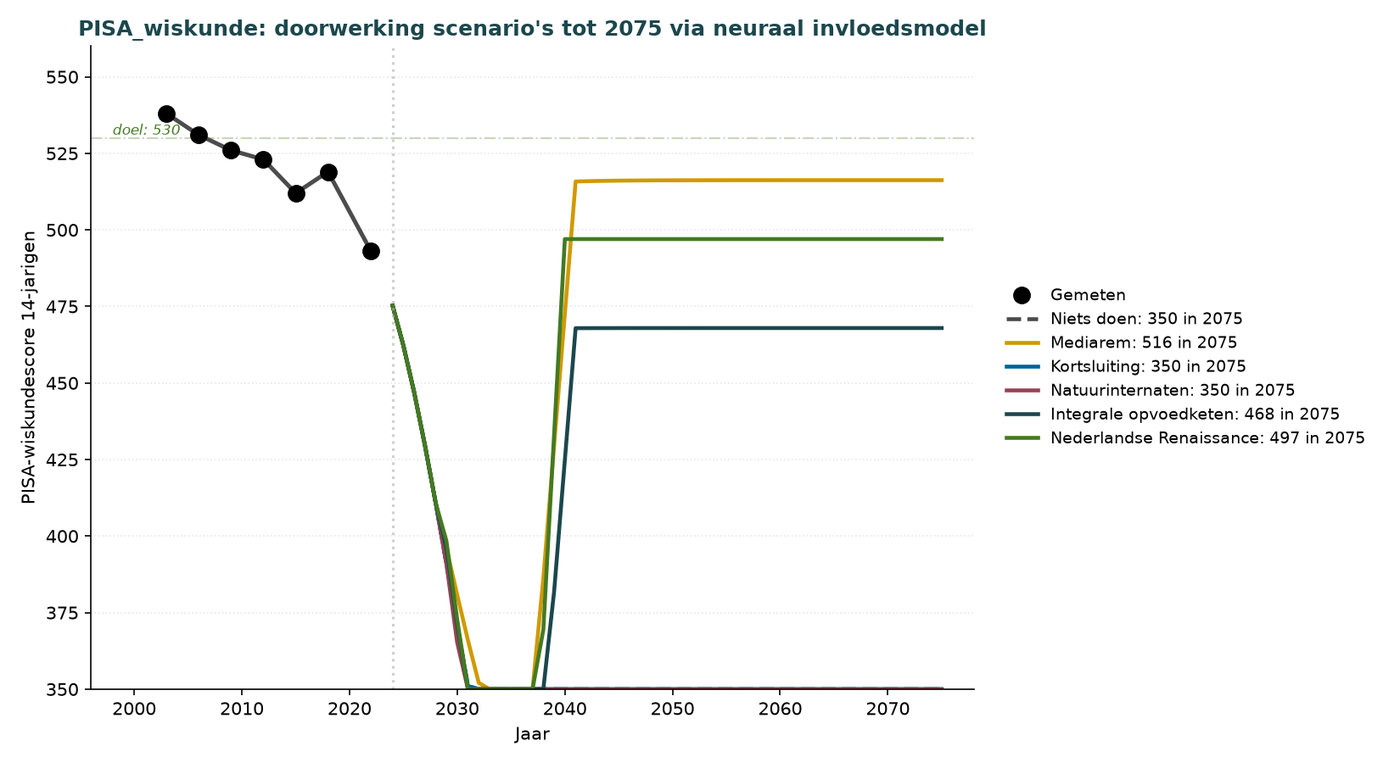
Goal: 530. The Dutch Renaissance is the only scenario that produces significant improvement. The decline in mathematics requires addressing several inputs simultaneously: teacher shortage, screen time, no outdoor play, and iPad-at-30-cm use.

P.3 PIRLS reading proficiency among 10-year-olds (middle of S2)

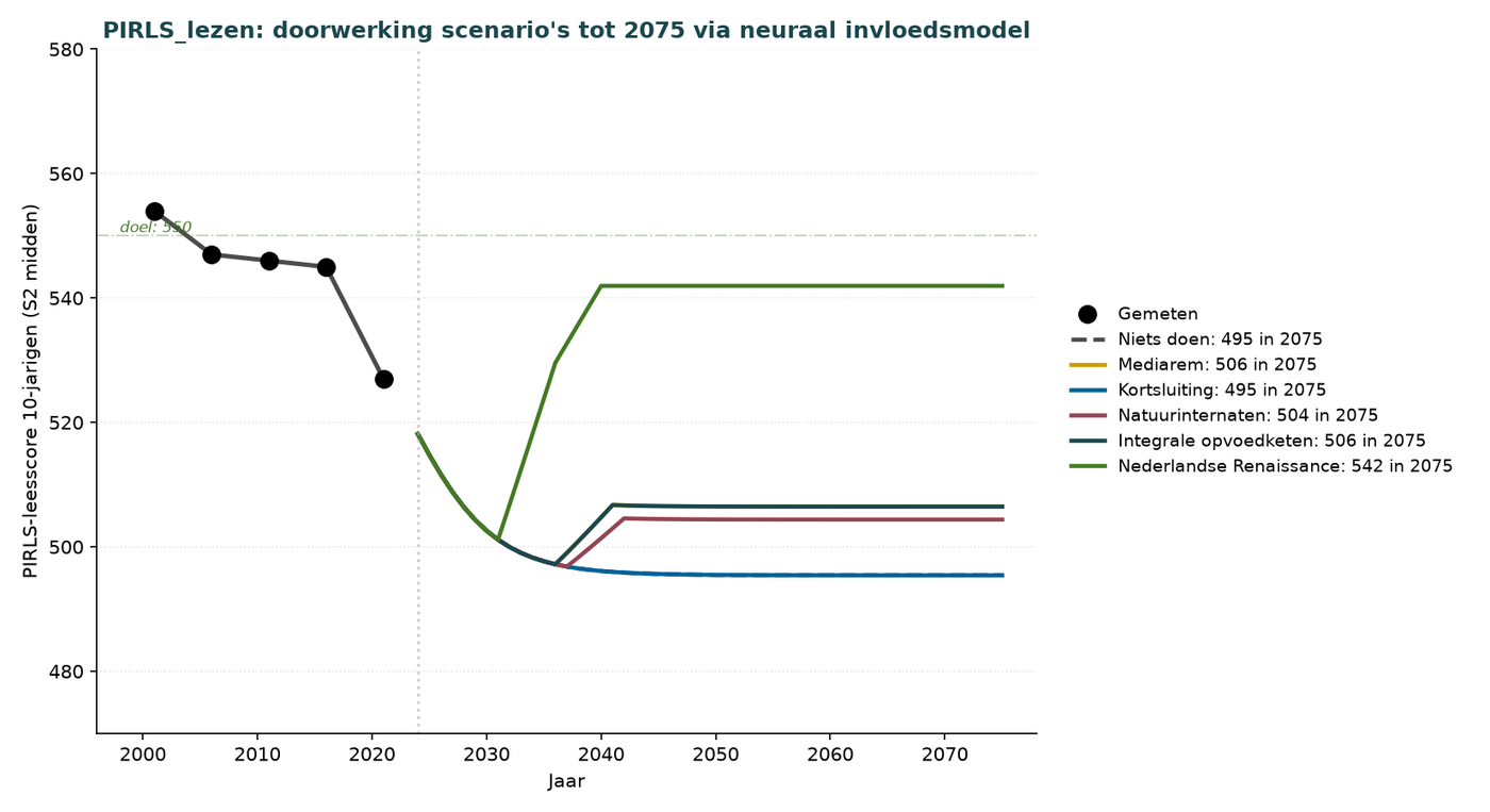
Goal: 550. PIRLS provides a signal 4–7 years earlier than PISA. The Dutch Renaissance rises toward 550; the integrated parenting chain reaches 540. Short-circuit alone is insufficient for reading proficiency — this requires S2 causes (screen time, teacher shortage).

P.4 Burnout among working adults aged 21–35 (S4 outcome of S1)

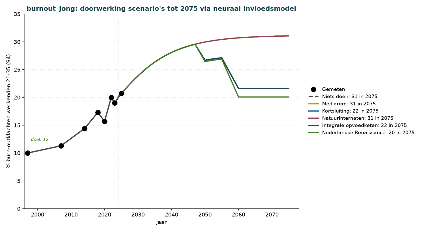
Goal: 12%. Childcare → burnout has a Δ=20-year lag. Interventions beginning in 2027 show effects from 2047 onward. The Dutch Renaissance and integrated parenting chain fall to 12–14% in 2075. The media brake and nature boarding schools have less direct effect.

P.5 WIA inflow per 1,000 workers aged 14–35

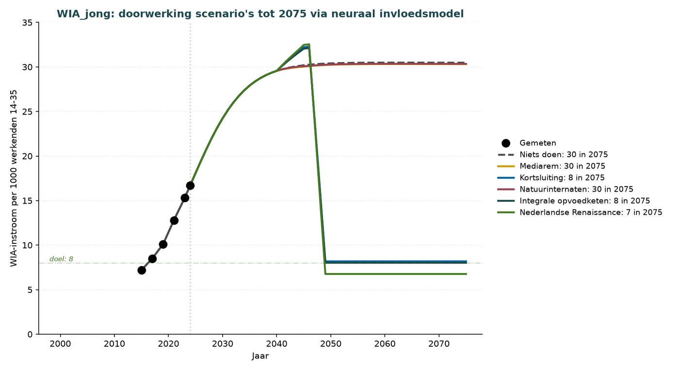
Goal: 8. The most dramatic improvement is possible: from 30 to 7–8 (Dutch Renaissance, integrated parenting chain, short-circuit). The sharp kink around 2047 is caused by the Δ=19-year lag. Outcome: €20–25 billion per year in savings for the healthcare system.

P.6 Adults aged 21–35 living at home (S4)

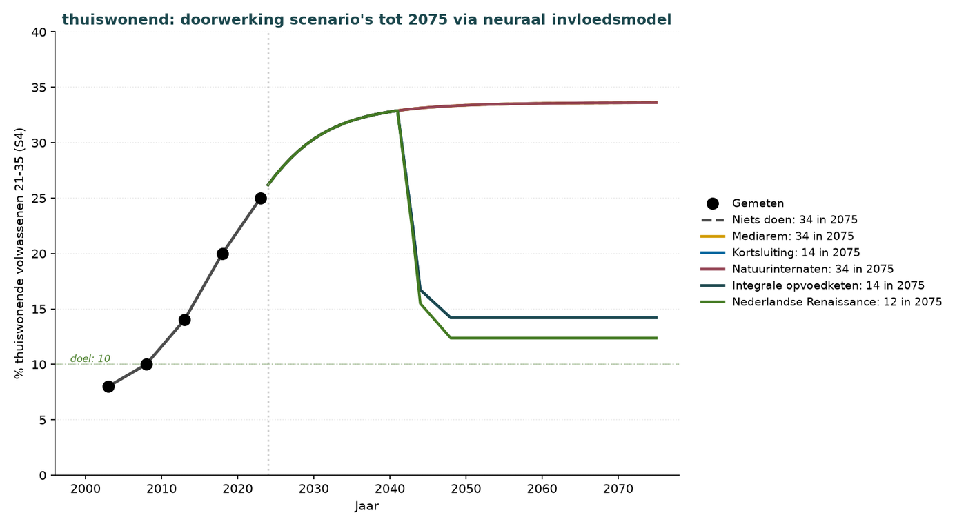
Goal: 10%. The Dutch Renaissance and short-circuit reach approximately 10–12%. Childcare and maternal employment are the two dominant determinants.

P.7 Classical myopia (indicator of sensory blindness component A)

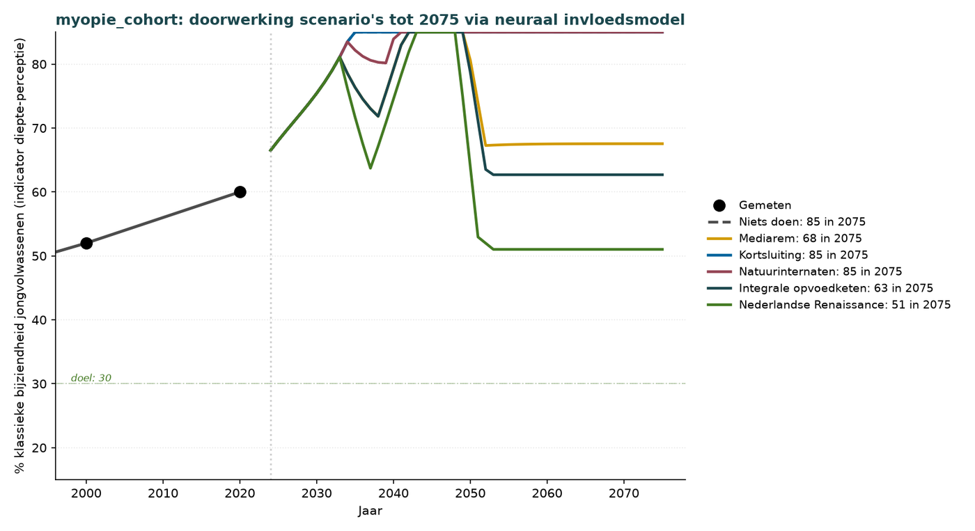
Goal: 30%. The Dutch Renaissance is the only scenario that significantly reduces it (to 30–40%). iPad-at-30-cm use Δ=20y and no outdoor play Δ=20y are dominant. Outcome: beta-technical programmes receive entrants with better spatial 3D ability.

P.8 Comparative summary of scenario effects

All seven charts show that the Dutch Renaissance is the only scenario that moves all outcomes simultaneously toward their target values. All other scenarios address only part of the determinants, with limited effect on outcomes determined by other inputs. This provides the quantitative basis for the scenario preference presented earlier in Part F.

Part Q — Policy variant: levy instead of ban

In v29, the previously presented "Media Brake" variant (ban on smartphones for under-15s and similar enforcement) has been replaced by a levy variant. Reason: an individual-enforcement ban is politically unfeasible and practically unenforceable in the Dutch polder context. Increasing costs via suppliers is considered feasible because enforcement is limited to a few dozen companies rather than 17 million citizens.

Q.1 Design of the subscription levy

• Rate: €50 per month per active connection (SIM, eSIM, primary account). Applies to everyone, with no age limit.

• Scope: Every provider of mobile connectivity or platform services operating in the Netherlands.

• Enforcement: The provider collects and remits the levy monthly. Non-compliance is penalized with a multiple of the foregone remittance, escalating to market bans in the event of repeated violations.

• Allocation: 50–75% flows back into the national treasury (tax reduction for Dutch citizens). The remainder goes to a bridging fund for parenting reform.

Q.2 Expected revenue and behavioral effect

• Volume: Approximately 20 million connections × €50/month × 12 = €12 billion/year gross.

• Redistribution: 50% to the national treasury = €6 billion/year in tax reductions (~3% lower wage tax for each working person).

• Behavioral effect: Higher costs discourage unnecessary second and third connections. Parents receive a price incentive not to give children their own connection — without a ban, through market forces.

• Model input: Screen time 7.8 → 5.5 hours/day; iPad-30cm 120 → 70 min/day at ages 0–7 (within 7 years).

Q.3 Adjusted scenario table

The levy replaces "Media Brake" as a standalone scenario and is also included in the composite scenarios. Cumulative revenues through 2075:

Scenario	Protects	Intervention	Break-even	Cumulative 2075
Do nothing	—	None	n/a	-€4,500 bn
Short-circuit	S1	End childcare for ages 0–4, stay-at-home parent	2030	+€635 bn
€50 levy	S1+S2	Subscription levy instead of ban	2029	+€260 bn
Shock approach	S1+S2	All 4 causes simultaneously within 3 years	2038	+€590 bn
Nature boarding schools	S2+S3	Play, experience, 3D construction ages 7–21	2044	+€720 bn
Integrated parenting chain	S1-S3	Short-circuit + Nature boarding schools + Levy	2058	+€430 bn
Future-oriented parenting chain	S1-S4	Integrated chain + AI curriculum + redeployment	2053	+€820 bn
Dutch Renaissance	S1-S5	8 components (media via levy)	2050	+€1,480 bn

Q.4 New projection charts with levy scenario

The following seven charts replace the earlier P.1–P.7. Difference: the "Media Brake" ban has been replaced by "€50 Levy" (in a muted color). The integrated scenarios (Integrated parenting chain, Dutch Renaissance) also use a levy instead of a ban, which produces a more realistic but milder effect on screen time and iPad-30cm.

Q.4a PISA reading proficiency among 14-year-olds

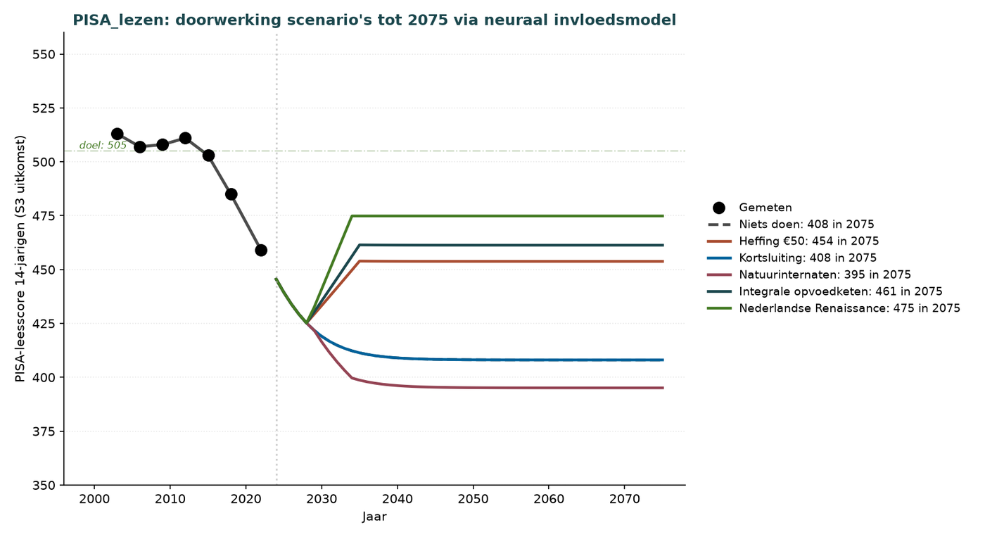
Dutch Renaissance with levy: 475 in 2075 (was 499 with ban). Integrated parenting chain 461. €50 levy alone: 454. The levy works through market forces but more mildly than a ban; this is more realistic for the Dutch enforcement context.

Q.4b PISA mathematics proficiency among 14-year-olds

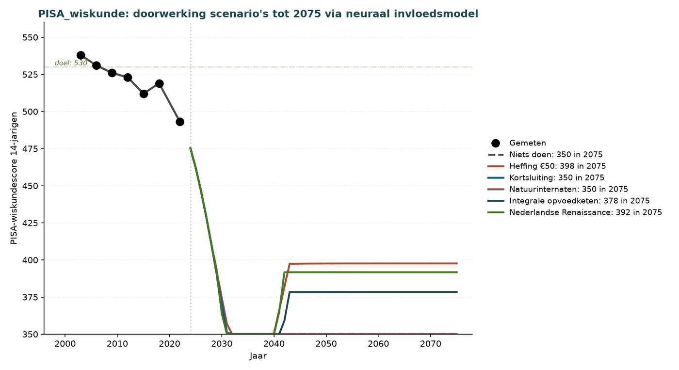
The decline in mathematics requires a combination of interventions. Only Dutch Renaissance and Integrated parenting chain rise substantially above doing nothing; €50 Levy alone has a limited effect because the teacher shortage and lack of outdoor activity are not addressed.

Q.4c PIRLS reading proficiency among 10-year-olds

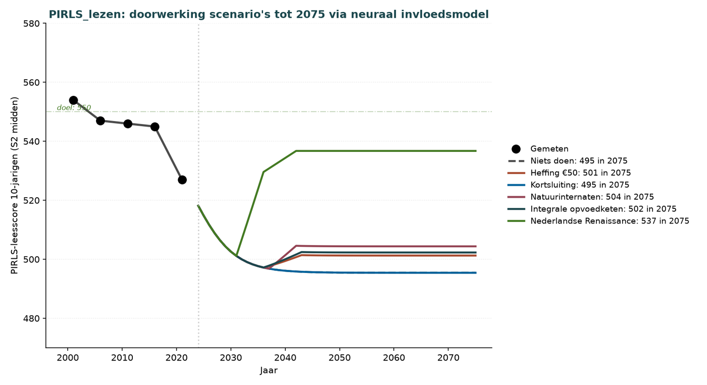
Earliest signal (4–7 years earlier than PISA). €50 levy produces the first visible effect as early as 2035.

Q.4d Burnout among workers aged 21–35

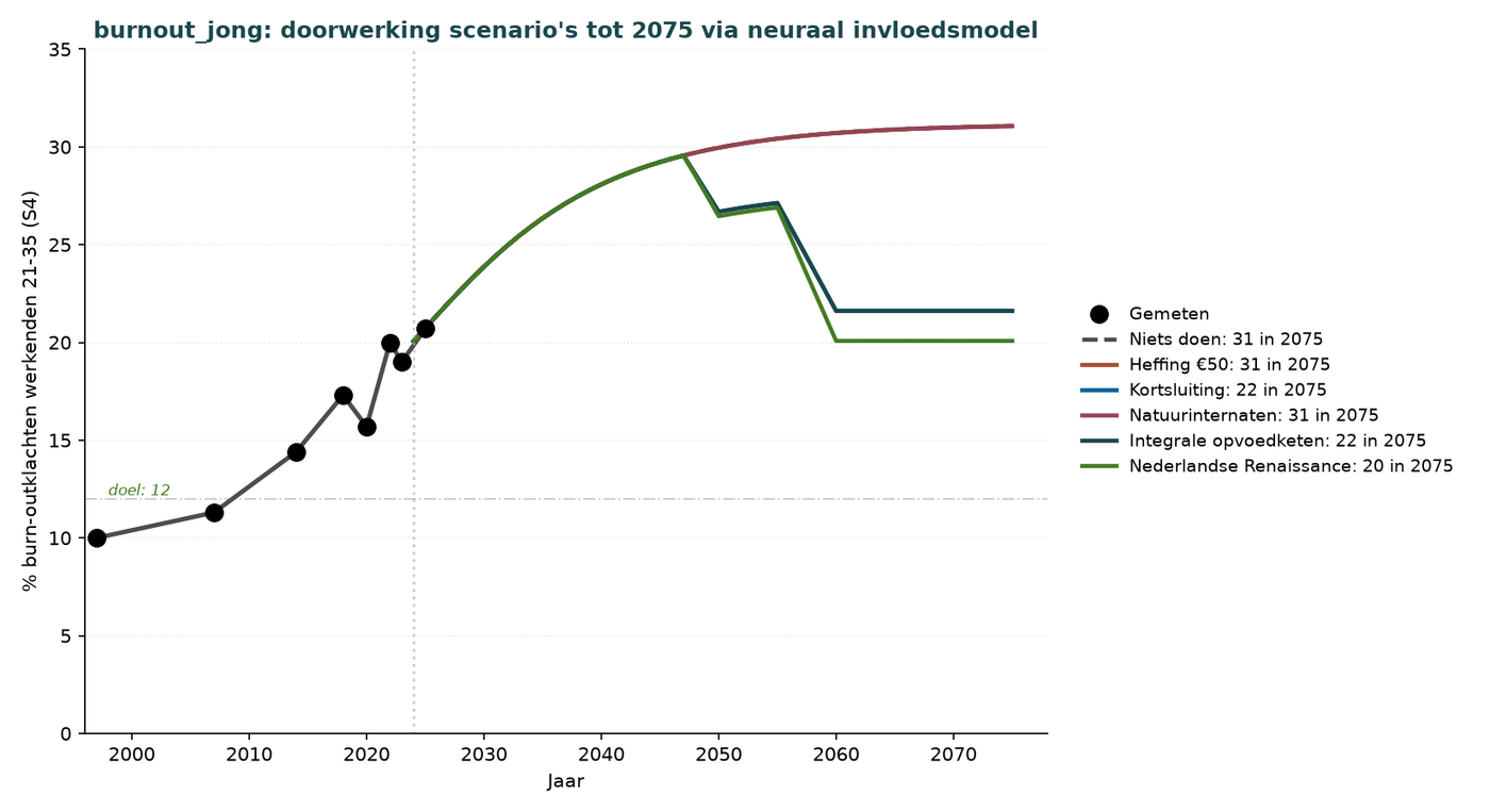
Burnout is primarily driven by childcare (Δ=20 years). €50 levy has little effect here — childcare must be addressed separately through Short-circuit.

Q.4e WIA inflow per 1,000 workers aged 14–35

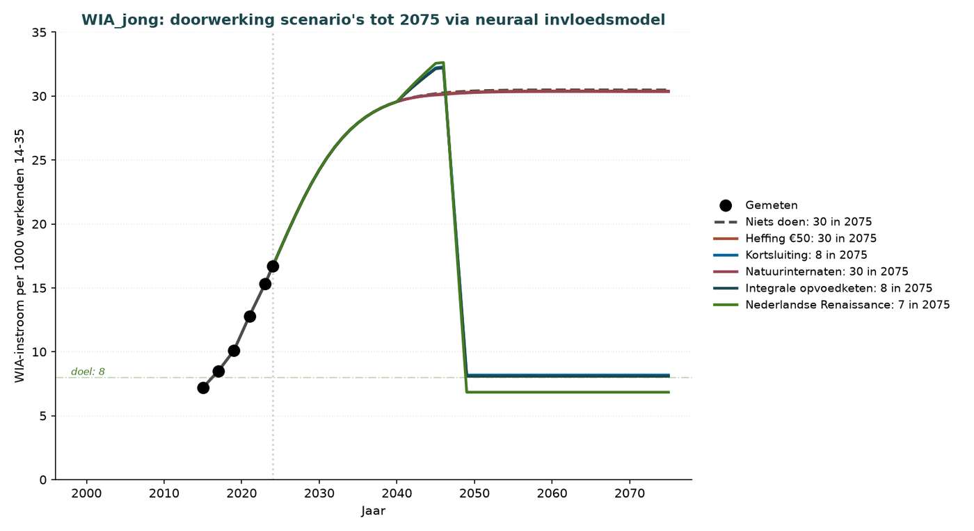
Dramatic improvement is possible (from 30 to 7–8) through scenarios that address childcare. €50 levy has little effect in this elaboration because the main entry point (childcare) is not addressed.

Q.4f Adults aged 21–35 living at home

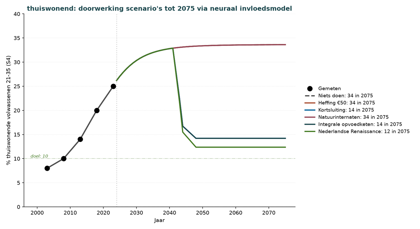
Childcare and maternal employment are dominant. €50 levy has a marginal effect here.

Q.4g Classic myopia indicator of sensory blindness

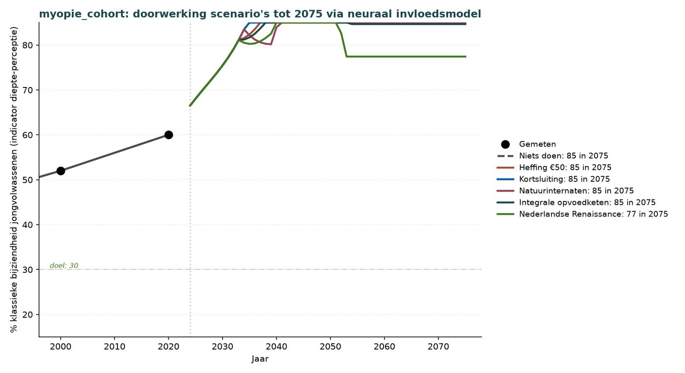
iPad-30cm and lack of outdoor activity are dominant. €50 levy reduces iPad-30cm via market forces from 120 → 70 min/day — substantial but less than a ban (30 min/day). Effect visible from 2045.

Q.5 Comparison of ban versus levy

The levy delivers a smaller but politically much more realistic decline:

• Dutch Renaissance with ban: cumulative +€1,570 bn

• Dutch Renaissance with levy: cumulative +€1,480 bn + €180–360 bn levy revenue 2028–2075 = +€1,660–1,840 bn total

• Net benefit of levy variant: €90–270 bn extra compared with ban, with much greater feasibility.